

The Class of Bar-Lev–Enis–Tweedie Distributions
notes
glm
exponential family
probability
programming
The class of power-variance family distributions jointly discovered by Bar-Lev and Enis, and Tweedie.

[M]athematics is about a world that is not quite the same as this real one outside the window, but it is just as obstinate. You can’t make things do what you want them to. [T]he very fact that I can’t just boss these mathematical entities around is evidence that they really exist. John Conway quoted in Roberts (2024).
1 Introduction
Everyone who’s modeled with GLMs has seen something like Table 1 describing the class of Tweedie Power Variance Family (PVF) distributions. This version is from the R statmod documentation.
| Distribution Name | Variance Function \(V(\mu)\) |
|---|---|
| Gaussian | \(\mu^0=1\) |
| Poisson | \(\mu\) |
| Compound Poisson, non-negative with mass at \(0\) | \(\mu^p\), \(1<p<2\) |
| Gamma | \(\mu^2\) |
| Inverse Gaussian | \(\mu^3\) |
| Stable, support on \(x>0\) | \(\mu^p\), \(p>2\) |
Table 1 is fascinating and raises several questions:
- What is a variance function?
- Why these distributions?
- Why this order?
- What about \(0<p<1\)? Or \(p<0\)?
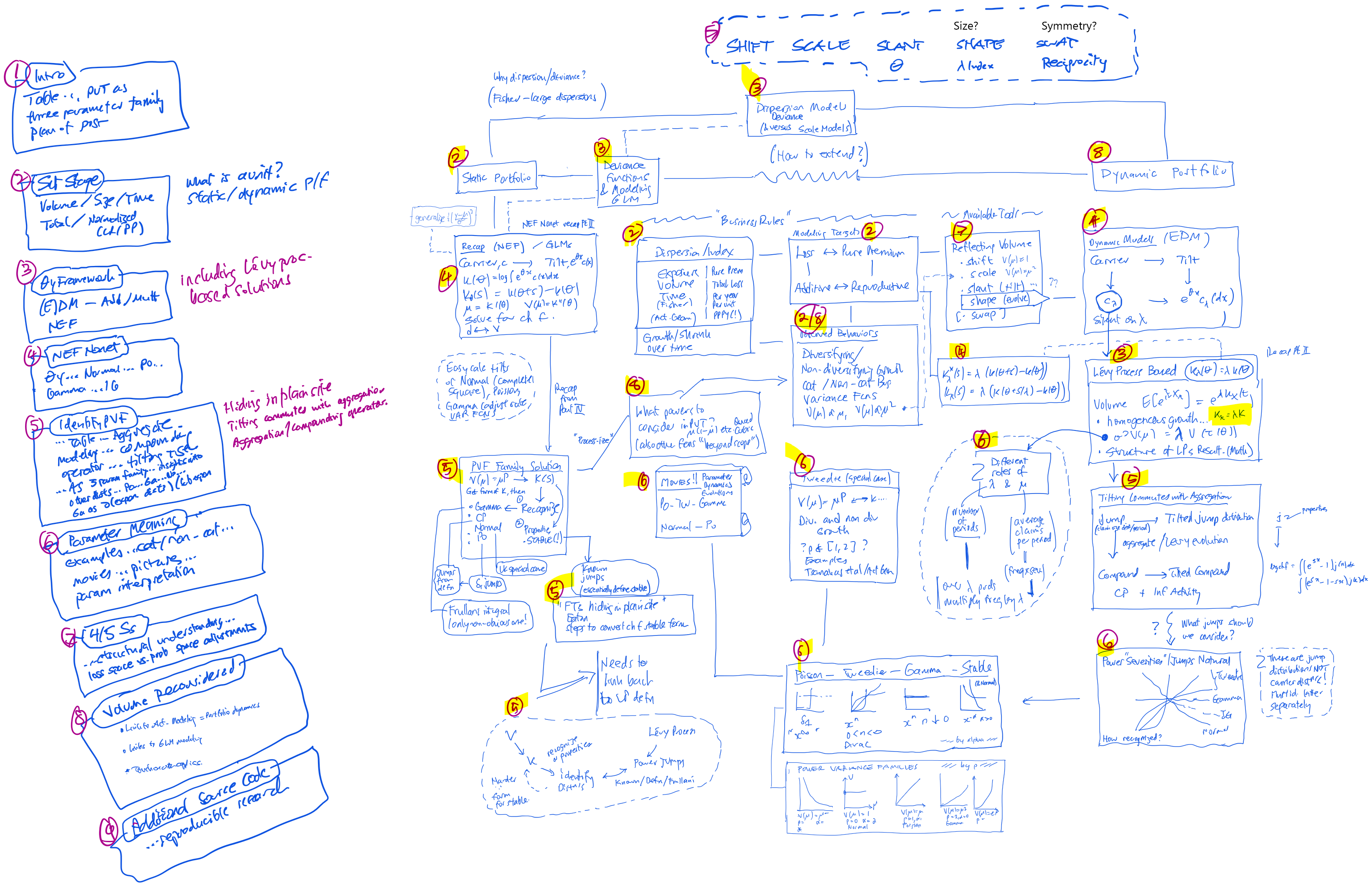
The Bar-Lev–Enis–Tweedie PVF (BLETPVF) turns out to be a large, three-parameter class of distributions including the Poisson, gamma, and Gaussian distributions. Table 2 shows the full story and this post will gradually explain all its entries. The theory of BLETPVFs is an example of Conway’s quote: you can control the starting definitions but not where things go from there! It is also an example of Mathematical Tourism. For me, this theory is like visiting and walking in the Lake District: beautiful views an unexpected connections. It’s like the crossing from Wast Water over the Sty Head Pass between Great Gable and Scafell Pike into the stunning valley of Borrowdale.
This post has eight main parts plus an supplement on the software.
- Introduction – you’re here.
- Setting the Stage
- Theoretic framework
- The NEF Nonet
- Identifying the BLETPVF distributions
- Parameter interpretation
- For Four/Five Esses
- Actuarial modeling reconsidered
- Software supplement
The post borrows heavily from my Four Part Series on Minimum Bias and Exponential Family Distributions
Themes: unreasonable effectiveness of maths; mapping real world to maths world; hiding in plain sight: looks different but actually the same, nature of actuarial modeling, what is a unit?
The post uses several tools from my aggregate software, Mildenhall (2024), including the FourierTools and the Tweedie classes. These leverage Fourier and Fast Fourier methods to estimate densities which have no closed form expression.
Terminology. The class of Bar-Lev–Enis–Tweedie power variance families consists of multiple natural exponential families. One family is the Tweedie Poisson-gamma compound distributions genus which we call a Tweedie distribution.
Bent’s uber paper ref Jørgensen (1987).
1.0.1 On the Title
Bar-Lev (2019) explains and provides supporting evidence that Bar-Lev and Enis (1986) was an “Independent and identical result” with the much-quoted (Jørgensen (1987)).
Rarely seen paper by Tweedie An index which distinguishes between some important exponential families published in “Statistics: Applications and new directions: Proc. Indian statistical institute golden Jubilee International conference (Vol. 579, pp. 579-604)”. Seems reasonable, hence the title.
1.1 The Full Story
We are going to explain and illustrate all the entries in Table 2.

Table 2 uses the following terms, all of which are explained in due course.
- The parameters \(p\) and \(\alpha\) are related by \(p=(\alpha-2)/(\alpha-1)\) and \(\alpha=(p-2)/(p-1)\), so \((1-p)(1-\alpha)=(p-1)(\alpha-1)=-1\). They are restricted to the range \([-\infty, 2]\).
- The distributions all have Lévy measure proportional to \(\dfrac{e^{\theta x}}{x^{\alpha+1}}\) when \(\alpha < 2\).
- \(\tau\) is the mean value mapping from the canonical parameter \(\theta\) to the mean parameter \(\mu\), the mean of the reproductive form.
- \(\Theta\) is the set of canonical parameters \(\theta\) so that \(\int e^{\theta y}c(y)\,dy< \infty\).
- \(\Omega\) is the mean domain, that is, the set of possible means.
- \(S\) is the support of the family. The trick here is distributions like the Poisson where \(\Omega\) is a strict subset of \(S\), because \(0\) is a legitimate observation but not an allowed mean.
- \(\Omega\) is a subset of \(C= \mathrm{conv}(S)^-\), the closure of the convex hull of \(S\).
- A natural exponential family is regular if the canonical parameter domain \(\Theta\) is open.
- It is steep when \(\Omega=C^\circ\), i.e., any value in interior of the convex closure of the support is a possible mean.
- The Levy \(1/2\)-stable distribution is a limit case of the inverse Gaussian as \(\theta\to 0\).
1.2 Lietfaden
1.3 Remember…
- Change alpha-p diagram to say Landau not Cauchy
- Have
Tweedieclass use Landau - Pitman and Pitman (2016) (Euler-Cauchy-Saalschütz integral - gamma with compensated exponential terms! Nice!
- Bar-Lev and Enis (1986) talks about reproducibility
- Bar-Lev, Bshouty, and Letac (1992) has a treatment of Tweedie family from perspective of self-decomposability.
- Swap or symmetry reciprocal?
- Letac (2004) dicusses \(V(\mu)=e^\mu\) as a variance function and reciprocity. States the NEF generated by a positive stable distribution whose parameter is in \((0, 1)\) has no reciprocal.
- Menn and Rachev (2006) covers the fancy Simpson’s method use of FFTs.
- The papers by Thomas Simon on unimodality look interesting too, e.g., Simon (2015).
- Books (all in Mendeley)
- Delong2021 - making more accessible
- Bar-Lev (2023) Cauchy -> Landau distribution
2 Setting the Stage
static portfolios — loss or normalized loss, pure premium, loss ratio — defining a unit or line — heterogeneous units — GLM modeling
2.1 Volume and Loss Aggregation
In modeling insurance losses, volume is a central consideration that affects both properties of the chosen loss distribution and statistical parameter inference. Volume reflects two dimensions: the size of an individual risk and the time horizon over which losses are accumulated. The resulting expected volume of losses depends on the product of exposure size and time horizon.
Size is measured using an exposure base. Units for auto, value for property, revenue or area for general liability, contract value for surety, payroll for workers compensation are examples. Each has issues. Ideally, size would be directly proportional to expected losses per unit of time, and we presume we have an ideal measure of size, despite essentially none actually existing. Call size \(z\).
Time horizon is measured in some time unit, usually years. However, the unit is an arbitrary choice ‒ an uncomfortable situation. Two time units are canonical: an instant and forever. The latter being too long, focus on the former. Turns out, it ties naturally to modeling in a multiple-state model or using a Lévy process, both of which are based on instantaneous transition rates @ REFs.
With volume in hand, modeling can look at total losses or losses per unit exposure (for a given time period), per time period (for a given exposure) or per unit per period. Losses are modeled by additive exponential dispersion models (EDMs) and pure premiums by reproductive EDMs. Some definitions are in order.
From Prob Models for Ins Research
Losses have a complicated, dynamic structure. An insurance portfolio’s loss depends on the expected loss rate and the length of time it is exposed, analogous to distance equals speed multiplied by time. Total losses \(L=L(e,t)\) over a period \((0,t]\) are a function of exposure and time. Exposure is measured in homogeneous units, each with the equal expected loss rates. What is the best way to model \(L(e,t)\)?
Is it reasonable to assume losses occur at a constant rate? Generally, not. Even for earthquake losses, where events appear perfectly random, the occurrence time influences losses. Did the loss occur during the commute, working hours, nighttime, or over a weekend? There are two ways to address this reality. One, over the time frame of an insurance policy the rate averages out and can be treated as constant. Two, use a time change to equalize the claim rate. The time change, called an operational time, runs time faster during high expected loss periods and slower during low. It provides the perfect clock against which to earn premium. As always, what matters is the deviation from expected. We proceed assuming a constant expected rate of claim occurrence, justified by either of these rationales.
If insured risks are independent, we could posit that losses over \((0,t_1+t_2]\) should have the same distribution as the sum of independent evaluations over \((0,t_1]\) and \((0,t_2]\). But there could be good reasons why this is not the case. Weather, for example, is strongly autoregressive: weather today is the best predictor of the weather tomorrow. Failure of independence manifests itself in an inter-insured and inter-temporal loss dependency or correlation. However, using common operational time and economic drivers can explain much of this correlation; see Avanzi, Taylor, and Wong (2016) and the work of Glenn Meyers on contagion.
Having stipulated caveats for expected loss rate and dependency, various loss models present themselves. A homogeneous model says \(L(e,t)=eR_t\) where \(R_t\) represents a common loss rate for all exposures. This model is appropriate for a stock investment portfolio, with position size \(e\) and stock return \(R_t\). It implies the CV is independent of volume.
A homogeneous model has \(L(e,t)\sim D(et, \phi)\), a distribution with mean \(m=et\) and additional parameters \(\phi\). A GLM then models \(m\) as a function of a linear combination of covariates, often with \(e\) as an offset. We can select the time period so that the expected loss from one unit of exposure in one period of time equals 1. In this model, time and exposure are interchangeable. The loss distribution of a portfolio twice the size is the same as insuring for twice as long. Thus we can merge loss rate and time into one variable \(\nu\) and consider \(L=L(\nu)\). If \(\nu\) is an integer then \(L(\nu)=\sum_{1\le i\le \nu} X_i\) where \(X_i\sim L(1)\) are independent. Therefore \(\mathsf{Var}(L(\nu))=\nu\mathsf{Var}(L(1))\) and the CV of \(L(\nu)\) is \(CV(L(1))/\sqrt{\nu}\). The CV of losses are not independent of volume, in contrast to the investment modeling paradigm. The actuary knows this: the shape of the loss distribution from a single policy (highly skewed, large probability of zero losses) is very different to the shape for a large portfolio (more symmetric, very low probability of zero losses.)
As always, reality is more complex. Mildenhall (2017) discusses five alternative forms for \(L(e,t)\). It shows that only a model with random operational time is consistent with NAIC Schedule P data, after adjusting for the underwriting cycle.
The focus of this section is to determine which distributions are appropriate for modeling homogeneous blocks with a constant loss rate relative to (operational) time. These distributions are used in predictive modeling for ratemaking and reserving, for example. Other applications, such as capital modeling and Enterprise Risk Management, model heterogeneous portfolios where understanding dependencies becomes critical. These are not our focus and are therefore ignored, despite their importance.
The ability to embed a static loss model \(L\) into a family, or stochastic process, of models \(L(\nu)\) appropriate for modeling different volumes of business over different time frames is an important concept that is introduced in this section. Dynamic modeling leads to a compound Poisson process and, more generally, a Lévy process. We begin by recalling the aggregate loss model of collective risk theory.
2.2 The Aggregate Loss Model
An aggregate loss model random variable has the form \(Y=X_1+\cdots +X_N\) where \(N\) models claim count (frequency) and \(X_i\) are independent, identically distributed (iid) severity variables. Aggregate loss models have an implicit time dimension: \(N\) measures the number of claims over a set period of time, usually one year. Aggregate loss models are the basis of the collective risk model and are central to actuarial science.
Expected aggregate losses equal expected claim count times average severity, \(\mathsf{E}[Y]=\mathsf{E}[N]\mathsf{E}[X]\). There is a tricky formula for the variance of \(Y\); here is an easy way to remember it. If \(X=x\) is constant then \(Y=xN\) has variance \(x^2\mathsf{Var}[N]\). If \(N=n\) is constant then \(X_1+\cdots +X_n\) has variance \(n\mathsf{Var}(X)\) because \(X_i\) are independent. The variance formula must specialize to these two cases and therefore, replacing \(n\) with \(\mathsf{E}[N]\) and \(x\) with \(\mathsf{E}[X]\), suggests \[ \mathsf{Var}(Y)=\mathsf{E}[X]^2\mathsf{Var}(N) + \mathsf{E}[N]\mathsf{Var}(X) \] is a good bet. By conditioning on \(N\) you can check it is correct.
2.3 Compound Poisson Distributions
A compound Poisson (CP) random variable is an aggregate loss model where \(N\) has a Poisson distribution. Let \(\mathsf{CP}(\lambda, X) = X_1+\cdots +X_N\) where \(N\) is a Poisson with mean \(\lambda\) and \(X_i\sim X\) are iid severities. We shall see that the Tweedie family is a CP where \(X_i\) have a gamma distribution.
By the results in the previous section \(\mathsf{E}[\mathsf{CP}(\lambda, X)]=\lambda\mathsf{E}[X]\). Since \(\mathsf{Var}(N)=\mathsf{E}[N]\) for Poisson \(N\) and \(\mathsf{Var}(X)=\mathsf{E}[X^2]-\mathsf{E}[X]^2\), we get \[ \mathsf{Var}(\mathsf{CP}(\lambda, X)) %= \mathsf{E}[N](\mathsf{Var}(X) + \mathsf{E}[X]^2) = \mathsf{E}[N]\mathsf{E}[X^2]. \]
CP distributions are a flexible and tractable class of distributions with many nice properties. They are the building block for almost all models of loss processes that occur at discrete times.
2.4 Diversifying and Non-Diversifying Insurance Growth
We want to understand the relationship between the variance of losses and the mean loss for an insurance portfolio as the mean varies, i.e., the variance function. Is risk diversifying, so larger portfolios have relatively lower risk, or are there dependencies which lower the effectiveness of diversification? Understanding how diversification scales has important implications for required capital levels, risk management, pricing, and the optimal structure of the insurance market. Let’s start by describing two extreme outcomes using simple CP models. Assume severity \(X\) is normalized so \(\mathsf{E}[X]=1\) and let \(x_2:=\mathsf{E}[X^2]\).
Consider \(\mathsf{CP}_1(\mu, X)\). The variance function is \(V(\mu)=\mathsf{Var}(\mathsf{CP}_1)=\mu x_2\), which grows linearly with \(\mu\). \(\mathsf{CP}_1\) models diversifying growth in a line with severity \(X\). Each risk is independent: increasing expected loss increases the expected claim count but leaves severity unchanged. \(\mathsf{CP}_1\) is a good first approximation to growth for a non-catastrophe exposed line.
Alternatively, consider \(\mathsf{CP}_2(\lambda, (\mu/\lambda)X)\) for a fixed expected event count \(\lambda\). Now, the variance function is \(V(\mu)=\mathsf{Var}(\mathsf{CP}_2)=\lambda(\mu/\lambda)^2x_2=\mu^2(x_2/\lambda)\) grows quadratically with \(\mu\). The distribution of the number of events is fixed, as is the case in a regional hurricane or earthquake cover. Increasing portfolio volume increases the expected severity for each event. \(\mathsf{CP}_2\) is a model for non-diversifying growth in a catastrophe-exposed line. It is the same as the position size-return stock investment model. Risk, measured by the coefficient of variation, is constant, equal to \(\sqrt{x_2/\lambda}\), independent of volume. This is a homogeneous growth model.
We will see in Part IV that the Tweedie family of compound Poisson distributions interpolates between linear and quadratic variance functions.
A more realistic model adds uncertainty in \(\mu\), resulting in a variance function of the form \(\mu(a+b\mu)\) which is diversifying for small \(\mu\) and homogeneous for larger \(\mu\).
2.5 The Moment Generating Function of a CP
Many useful properties of CP distributions are easy to see using MGFs. To compute the MFG of a CP we first to compute the MGF of a Poisson distribution. We need two facts: the Poisson probability mass function \(\mathsf{Pr}(N=n)=e^{-\lambda}\lambda^n/n!\) and the Taylor series expansion of the exponential function \(e^x=\sum_{n\ge 0} x^n/n!\). Then \[ \begin{aligned} M_N(t) &=\mathsf{E}[e^{tN}] \\ &= \sum_{n\ge 0} e^{tn} \frac{e^{-\lambda} \lambda^n}{n!} \\ &= e^{-\lambda} \sum_{n\ge 0} \frac{(e^{t} \lambda)^n}{n!} \\ &= e^{-\lambda} e^{\lambda e^t} \\ &= \exp(\lambda(e^t-1)) \end{aligned} \] We can now compute the MGF of \(\mathsf{CP}(\lambda,X)\) using conditional expectations and the identity \(x^n=e^{n\log(x)}\): \[ \begin{aligned} M_{\mathsf{CP}(\lambda,X)}(t) &=\mathsf{E}[e^{t\mathsf{CP}(\lambda,X)}] \\ &=\mathsf{E}_N[\mathsf{E}_X[e^{t(X_1+\cdots X_N)}\mid N]] \\ &= \mathsf{E}_N[(\mathsf{E}_X[e^{tX}])^N] \\ &= \mathsf{E}_N[M_X(t)^N] \\ &= \mathsf{E}_N[e^{N\log(M_X(t))}] \\ &= M_N(\log(M_X(t))) \\ &= \exp(\lambda(M_X(t)-1)). \end{aligned} \] A Poisson variable can be regarded as a CP with degenerate severity \(X\equiv 1\), which has MGF \(e^t\). Thus the formula for the MGF of a CP naturally extends the MGF of a Poisson variable.
An example showing the power of MGF methods comes from the problem of thinning. We want to count the number of claims excess \(x\) where ground-up claims have a distribution \(\mathsf{CP}(\lambda, X)\). Take severity to be a Bernoulli random variable \(B\) with \(\mathsf{Pr}(B=1)=\mathsf{Pr}(X>x)=p\) and \(\mathsf{Pr}(B=0)=1-p\). \(B\) indicates if a claim exceeds \(x\). \(\mathsf{CP}(\lambda, B)\) counts the number of excess claims. It is called a thinning of the original Poisson. It is relatively easy to see that \(\mathsf{CP}(\lambda, B) \sim \mathrm{Poisson}(\lambda p)\) using the conditional probability formula \(\mathsf{Pr}(\mathsf{CP}=n)=\sum_{k\ge n}\mathsf{Pr}(\mathsf{CP}=n\mid N=k)\mathsf{Pr}(N=k)\) (exercise). But it is very easy to see the answer using MGFs. By definition \(M_B(t)=(1-p)+pe^t\), and therefore \[ \begin{aligned} M_{\mathsf{CP}}(t) &=M_N(\lambda(M_B(t)-1)) \\ &=M_N(\lambda((1-p+pe^t-1))) \\ &=\exp(\lambda p(e^t-1)). \end{aligned} \]
The MGF of a mixture is the weighted average of the MGFs of the components. If \(\bar X\) is a \(p_1,p_2\), \(p_1+p_2=1\), mixture of \(X_1\) and \(X_2\), so \(F_{\bar X}(x)=p_1F_1(x) + p_2F_2(x)\), then \[ \begin{aligned} M_{\bar X}(t)&=\int e^{tx}\left(p_1f_{X_1}(x) +p_2f_{X_2}(x)\right)\,dx\\ &=p_1\int e^{tx}f_{X_1}(x)\,dx + p_2\int e^{tx} f_{X_2}(x)\,dx\\ &= p_1M_{X_1}(t) + p_2M_{X_2}(t). \end{aligned} \] This fact allows us to create discrete approximation CPs and convert between a frequency-severity and a jump severity distribution view. It is helpful when working with catastrophe model output.
2.6 The Addition Formula
CP distributions satisfy a simple addition formula \[ \mathsf{CP}(\lambda_1, X_1) + \mathsf{CP}(\lambda_2, X_2) \sim \mathsf{CP}(\lambda, \bar X) \] where \(\lambda=\lambda_1 + \lambda_2\) and \(\bar X\) is a mixture of independent \(X_1\) and \(X_2\) with weights \(\lambda_1/\lambda\) and \(\lambda_2/\lambda\). The addition formula is intuitively obvious: think about simulating claims and remember two facts. First, that the sum of two Poisson variables is Poisson, and second, that to simulate from a mixture, you first simulate the mixture component based on the weights and then simulate the loss from the selected component.
It is easy to demonstrate the the addition formula using MGFs: \[ \begin{aligned} M_{\mathsf{CP}(\lambda_1, X_1) + \mathsf{CP}(\lambda_2, X_2)}(t) &= M_{\mathsf{CP}(\lambda_1, X_1)}(t)\,M_{\mathsf{CP}(\lambda_2, X_2)}(t) \\ &= \exp(\lambda_1(M_{X_1}(t)-1))\exp(\lambda_2(M_{X_2}(t)-1)) \\ &= \exp(\lambda([(\lambda_1/\lambda)M_{X_1}(t)+ (\lambda_1/\lambda)M_{X_2}(t)] -1)) \\ &= \exp(\lambda(M_{\bar X}(t) -1)) \\ &= M_{\mathsf{CP}(\lambda, \bar X)}(t). \end{aligned} \] The addition formula is the MGF for a mixture in reverse. To sum of multiple CPs you sum the frequencies and form the frequency-weighted mixture of the severities.
The addition formula is handy when working with catastrophe models. catastrophe models output a set of events \(i\), each with a frequency \(\lambda_i\) and a loss amount \(x_i\). They model the number of occurrences of each event using a Poisson distribution. Aggregate losses from the event \(i\) are given by \(\mathsf{CP}(\lambda_i, x_i)\) with a degenerate severity.
It is standard practice to normalize the \(\lambda_i\), dividing by \(\lambda=\sum_i\lambda_i\), and form the empirical severity distribution \(\hat F(x)=\sum_{i:x_i\le x} \lambda_i/\lambda\). \(\hat F\) is the \(\lambda_i\) weighted mixture of the degenerate distribution \(X_i=x_i\). By the addition formula, aggregate losses across all events are \(\mathsf{CP}(\lambda, \hat X)\) where \(\hat X\) has distribution \(\hat F\).
2.7 Lévy Processes and the Jump Size Distribution
The CP model of insurance losses is very compelling. The split into frequency and severity mirrors the claims process. However, we could take a different approach. We could specify properties an insurance loss model must have, and then try to determine all distributions satisfying those properties. In the process, we might uncover a new way of modeling losses. The latter approach has been used very successfully to identify risk measures. For example, coherent risk measures emerge as those satisfying a set of axioms.
As we discussed in the introduction, in a basic insurance model losses occur homogeneously over time at a fixed expected rate. As a result, losses over a year equal the sum of twelve identically distributed monthly loss variables, or 52 weekly, or 365 daily variables, etc. If the random variable \(Y_1\) represents losses from a fixed portfolio insured for one year, then for any \(n\) there are independent, iid variables \(X_i\), \(i=1,\dots, n\) so that \(Y_1=X_1 + \dots + X_n\). Random variables with this divisibility property for every \(n\ge 1\) are called infinitely divisible (ID). The Poisson, normal, gamma, negative binomial, lognormal, and Pareto distributions are all ID. This is obvious for the first four from the form of their MGFs. For example, the Poisson MGF shows \[ e^{\lambda(e^t-1)}=\{e^{\frac{\lambda}{n}(e^t-1)}\}^n \] so the Poisson is a sum of \(n\) Poisson variables for any \(n\). The same applies to a CP. Proving the lognormal or Pareto is ID is much trickier. A distribution with finite support, such as the uniform or binomial distributions, is not ID. A mixture of ID distributions is ID if the mixture distribution is ID.
Any infinitely divisible distribution \(Y\) can be embedded into a special type of stochastic process called a Lévy process so that \(Y\) has the same distribution as \(Y_1\). The process \(Y_t\) shows how losses occur over time, or as volume increases, or both. \(Y_t\) is a Lévy process if it has independent and identically distributed increments, meaning the distribution of \(Y_{s+t}-Y_s\) only depends on \(t\) and is independent of \(Y_s\). Lévy processes are Markov processes: the future is independent of the past given the present. The Lévy processes representation is built-up by determining the distribution of \(Y_\epsilon\) for a very small \(\epsilon\) and then adding up independent copies to determine \(Y_t\). The trick is to determine \(Y_\epsilon\).
Lévy processes are very well understood. See Sato (1999) for a comprehensive reference. They are the sum of a deterministic drift, a Brownian motion, a compound Poisson process for large losses, and a process that is a limit of compound Poisson processes for small losses. All of four components do not need to be present. Insurance applications usually take \(Y_t\) to be a compound Poisson process \(Y_t=X_1+\cdots + X_{N(t)}\), where \(X_i\) are iid severity variables and \(N(t)\) is a Poisson variable with mean proportional to \(t\).
When a normal, Poisson, gamma, inverse Gaussian, or negative binomial distribution is embedded into a Lévy processes, all the increments have the same distribution, albeit with different parameters. This follows from the form of their MGFs, following the Poisson example above. But it is not required that the increments have the same distribution. For example, when a lognormal distribution is embedded the divided distributions are not lognormal—it is well known (and a considerable irritation) that the sum of two lognormals is not lognormal.
The structure of Lévy processes implies that the MGF of \(X_t\) has the form \[ \mathsf{E}[e^{sX_t}] = \exp(t\kappa(s)) \] where \(\kappa(s)=\log\mathsf{E}[e^{sX_1}]\) is cumulant generating function of \(X_1\). To see this, suppose \(t=m/n\) is rational. Then, by the additive property \(\mathsf{E}[e^{sX_{m/n}}]=\mathsf{E}[e^{sX_{1/n}}]^m\) and \(\mathsf{E}[e^{sX_1}]=\mathsf{E}[e^{sX_{1/n}}]^n\), showing \(\mathsf{E}[e^{sX_1}]^{1/n}=\mathsf{E}[e^{sX_{1/n}}]\). Thus \(\mathsf{E}[e^{sX_{m/n}}]=\mathsf{E}[e^{sX_{1}}]^{m/n}\). The result follows for general \(t\) by continuity. Therefore, the cumulant generating function of \(X_t\) is \(\kappa_t(s) = t \kappa(s)\).
3 Theoretical Framework
dispersion models — DM and EDM — NEF — additive and reproductive
Figure 1 shows the relationship between dispersion models, regular proper DMs (not discussed), and reproductive and additive Exponential DMs. When the scale index is known an EDM becomes a NEF.
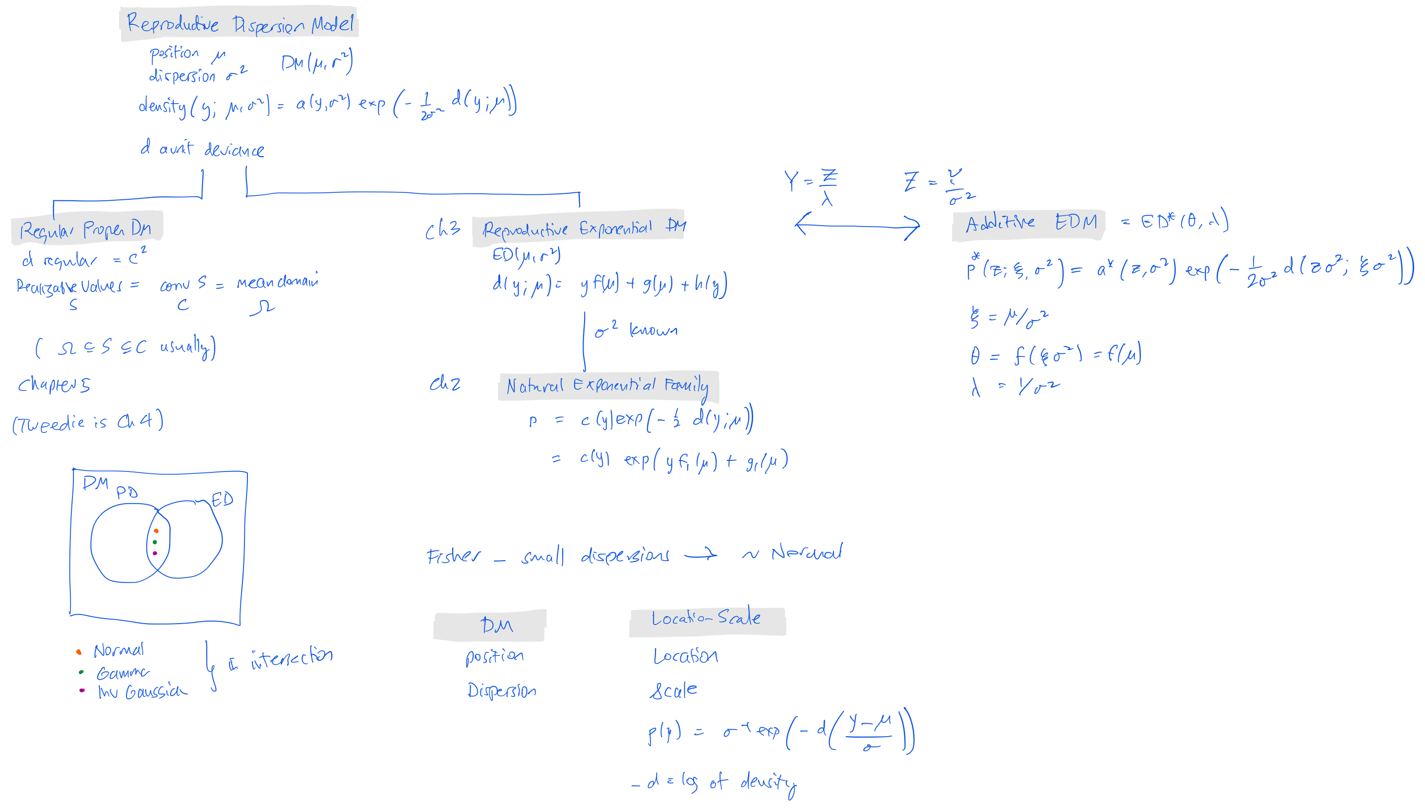
3.1 Dispersion Models
We start by defining some terminology around dispersion models (DMs). The idea is to generalize the normal with density \[ p(y; \mu, \sigma^2) = \frac{1}{\sqrt{2\pi\sigma^2}}\exp\left(-\frac{1}{2\sigma^2}(y-\mu)^2 \right). \]
Dispersion models have reproductive and additive parameterizations.
In the reproductive form, the natural parameter \(\theta\) and the canonical statistic \(T(X)\) are structured so that sums of independent observations preserve the distributional form. If \(X_1, \dots, X_n\) are i.i.d. from an exponential family distribution, their sufficient statistic \(T_n = \sum_{i=1}^{n} T(X_i)\) follows the same type of distribution with an updated natural parameter. The logic behind the name “reproductive” is that the sum of i.i.d. observations has the same distributional form, meaning the distribution is “reproduced” under summation.
Reproductive: The sum of independent observations retains the same family of distributions.
With the additive parameterization, the focus is on rewriting the exponential family form in a way that makes the natural parameter explicitly additive when combining independent observations. The key idea is that when summing independent variables, the natural parameters (or a transformation of them) add directly. The name “additive” comes from the fact that the parameter transformation aligns with addition when combining independent samples.
Additive: The natural parameters (or their transformation) combine via addition.
3.1.1 Reproductive dispersion models
A reproductive dispersion model with position parameter \(\mu\) and dispersion parameter \(\sigma^2\) is a family with density of the form \[ p(y;\mu, \sigma^2) = a(y;\sigma^2)\exp\left( -\frac{1}{2\sigma^2} d(y;\mu) \right) \] for \(y\in C\subset\mathbf R\) and \(\sigma^2>0\), where \(d\) is a deviance function. Deviance functions generalize \((y-\mu)^2\): \(d(y\mu) > 0\) for \(y\not=\mu\) and \(d(y;y)=0\), see Section 4.8. The model is called an exponential dispersion model \(\mathrm{ED}(\mu, \sigma^2)\) if the deviance has the form \[ d(y;\mu) = yf(\mu) + g(\mu) + h(y). \] The parameter \(\mu\) is called the mean value parameter and \(\sigma^2\) the dispersion parameter.
3.1.2 Natural exponential families
A natural exponential family (NEF) \(\mathrm{NE}(\mu)\) is a family of densities of the form \[ c(y)\exp\left( -\frac{1}{2} d(y;\mu) \right). \] A reproductive EDM with \(\sigma^2\) known is a NEF. In that case the density is \[ c_1(y)\exp\left( yf_1(\mu) + g_1(\mu) \right) \] for suitable \(f_1\), \(g_1\), subsuming the \(\exp(h(y))\) factor and \(c(y)\).
3.1.3 Additive dispersion models
The additive form is \[ Z= \frac{Y}{\sigma^2} = \lambda Y \] where \(\lambda = 1 / \sigma\) is called an additive exponential dispersion model. This is written \(Z\sim\mathrm{ED}^*(\theta,\lambda)\) where \(\theta=f(\mu)\) and \(\lambda=1/\sigma^2\). The parameters \(\theta\) is called the canonical parameter and \(\lambda > 0\) the index parameter.
3.2 Volume and Loss Aggregation with EDMs
The choice of loss or pure premium aggregation determines whether losses are viewed in total or on a per-policy-per-period (what health actuaries call pppy, per person per year) averages, leading naturally to two related sets of models.
Total Losses using an Additive Model. In many actuarial applications, the total loss across multiple policies or over an extended period is the primary object of interest. When losses are aggregated, the natural structure is additive, \(\mathrm{ED}^*(\theta, \lambda)\). The sum should retain the same distributional form: \[ \sum_i \mathrm{ED}^*(\theta, \lambda_i) \sim \mathrm{ED}^*\left(\theta, \sum_i\lambda_i\right). \] The classic example is a compound Poisson (CP) model, where \(\lambda_i\) determine expected claim count of different units and \(\theta\) determines the per claim severity distribution. CP models with the same severity add by adding expected frequencies, \(\lambda_i\).
Average Loss per Period using a Reproductive Model. In other settings, particularly in experience rating or loss ratio analysis, the focus shifts to per-unit per-period loss measures, \(\mathrm{ED}^*(\theta, \lambda)/\lambda\) calling for the reproductive structure, \(Y=\mathrm{ED}(\mu, \sigma^2)\). The mean \(\mu\) refers to the per-unit-per-period expected loss. The statistical properties of \(Y\) vary with context. If the unit is all losses from Mega Corp. Inc., over a year then \(\mu\) could be very large and have a tight distribution (\(\mu\) large, \(\sigma^2\) small). Conversely, for My Umbrella Policy with a $25M limit above $1M primary policies, losses per year have a very low mean but broad distribution (\(\mu\) small, \(\sigma^2\) large). However, in both cases actuaries know that the average becomes less dispersed as more units (measured in like policy-years) are combined. Pure premiums and loss ratios combine using a weighted average approach. If the distribution for one policy-year has parameters \(\mu\) and \(\sigma^2\) and distribution \(\mathrm{ED}(\mu, \sigma^2)\), then the per policy-per year average of \(n_i\) policy-years of identical exposures has distribution \(\mathrm{ED}(\mu, \sigma^2 / n_i)\) and this is an assumption! These should combine \[ \frac{1}{n}\sum_i \mathrm{ED}\left(\mu, \frac{\sigma^2}{n_i}\right) \sim \mathrm{ED}\left(\mu, \frac{\sigma^2}{n} \right) \] where \(n=\sum_i n_i\) is the total exposure modeled. The classic example here is adding normals derived as averages from different sample sizes, where the variance of the average from \(n_i\) observations equals \(\sigma^2/n_i\).
Exponential dispersion models support both views—total and per-unit losses—through its underlying structural properties.
3.3 Exponential Dispersion Models
An exponential dispersion model (EDM) is a collection of NEFs whose generator densities form a Lévy process. There are two kinds of EDM.
Let \(Z_\nu\) be a Lévy process with density \(c(y;\nu)\). The variable \(\nu\) is called the index parameter. \(\nu\) is used in place of \(t\) to be agnostic: it can represent expected loss volume or time or a combination. In the finite variance case, the distribution of \(Z_\nu\) becomes less dispersed as \(\nu\) increases. Therefore it is natural to define \(1/\nu\) as a dispersion parameter. For Brownian motion the dispersion parameter is usually denoted \(\sigma^2\). Throughout \(\sigma^2=1/\nu\) and the two notations are used inter-changeably. \(Z_\nu\) and \(\nu Z_1\) have the same mean, but the former has varying coefficient of variation \(\mathrm{CV}(Z_1)/\sqrt{\nu}\) and the latter a constant CV. \(Z_\nu\) is more (\(\nu<1\)) or less (\(\nu>1\)) dispersed than \(Z_1\). The difference between \(Z_\nu\) and \(\nu Z_1\) are illustrated in the lower two panels of Figure 11.
The first kind of EDM is an additive exponential dispersion model. It comprises the NEFs associated with the generator distribution \(Z_\nu\). It has generator density \(c(z; \nu)\) and cumulant generator \(\kappa_\nu(\theta)=\nu\,\kappa(\theta)\). Its members are all exponential tilts of \(c(z; \nu)\) as \(\nu\) varies. A representative distribution \(Z \sim \mathrm{DM}^*(\theta, \nu)\) has density \[ c(z;\nu) e^{\theta z - \nu\,\kappa(\theta)}. \] As \(\nu\) increases, the mean of the generator distribution increases and it becomes less dispersed. The same is true for \(Z\). The cumulant generating function of \(Z\) is \[ K(t;\theta, \nu) = \nu(\kappa(t+\theta) - \kappa(\theta)). \] If \(Z_i\sim \mathrm{DM}^*(\theta, \nu_i)\) and \(Z=\sum Z_i\), then the cumulant generating function for \(Z\) is \((\sum_i \nu_i)(\kappa(t+\theta) - \kappa(\theta))\) showing \(Z\) has distribution \(\mathrm{DM}^*(\theta, \sum_i \nu_i)\) within the same family, explaining why the family is called additive. Additive exponential dispersions are used to model total losses.
The second kind of EDM is a reproductive exponential dispersion model. It comprises the NEFs associated with the generator distribution of \(Y_\nu=Z_\nu/\nu\). \(Y_\nu\) has a mean independent of \(\nu\), but this independence is illusionary since the mean can be adjusted by re-scaling \(\nu\). In the finite variance case, \(Y_\nu\) has decreasing CV as \(\nu\) increases. The densities of \(Y\) and \(Z\) are related by \(f_Y(y)=\nu f_Z(\nu y)\). Hence a representative has density \[ f_Y(y)=\nu c(\nu y, \nu)e^{\nu(\theta y - \kappa(\theta))}. \] The cumulant generating function of \(Y\) is \[ K(t;\theta, \nu) = \nu(\kappa(t/\nu+\theta) - \kappa(\theta)). \]
To end this section, let’s work out the impact of tiling on the Lévy measure \(J\). In the last section, we saw that the cumulant generator of \(Z\) has the form \[ \kappa(\theta) = a\theta + \int_0^1 (e^{\theta x} -1 -\theta x)\,j(x)\,dx + \int_1^\infty (e^{\theta x} -1)\,j(x)\,dx \] where \(a\) is a location (drift) parameter. Rather than split the integral in two, write it as \[ \int_0^\infty (e^{\theta x} -1 -\theta x1_{(0,1)}(x))\,j(x)\,dx. \] where \(1_{(0,1)}\) is the indicator function on \((0,1)\). The \(\theta\)-tilt of \(Z\) has cumulant generating function \[ \begin{aligned} K_\theta(s) &= \kappa(s+\theta) - \kappa(\theta) \\ &= as + \int_0^\infty (e^{(s+\theta) x} - e^{\theta x} - s x1_{(0,1)}(x))\,j(x)\,dx \\ &= as + \int_0^\infty (e^{s x} - 1 - se^{-\theta x} x1_{(0,1)}(x))\, e^{\theta x}j(x)\,dx. \end{aligned} \] The factor \(e^{-\theta x}\) in the compensation term can be combined with \(1_{(0,1)}\), resulting in an adjustment to the drift parameter. Thus the Lévy distribution of the tilted distribution is \(e^{\theta x}j(x)\).
3.4 Connection to GLM modeling
We’re thinking the underlying units are characterized by a single size of loss distribution that is similar to a severity curve. DETAILS
4 The NEF Nonet
carrier or generating density — exponential tilting — cumulant generator — cumulant generating function — mean value mapping — variance function — log likelihood — unit deviance — density from deviance — Lévy distribution families
Material from The NEF Circle/Nonet.
This section describes the NEF Nonet which gives nine ways to define a NEF Section 3.1. The EDM index parameter is assumed known in a NEF.

4.1 The Generating Density
A generator or carrier is a real valued function \(c(y)\ge 0\). (The argument is \(y\) for historical reasons, where \(y\) represented as response.) If \(c\) is a probability density, \(\int c(y)dy = 1\), then it is called a generating density. However, \(\int c(y)dy\neq 1\) and even \(\int c(y)dy=\infty\) are allowed. The generating density sits at the top of the circle, reflecting its fundamental importance.
How can we create a probability density from \(c\)? It must be normalized to have integral 1. Normalization is not possible when \(\int c(y)dy=\infty\). However, it will be possible to normalize the adjusted generator \(c(y)e^{\theta y}\) when its integral is finite. To that end, define \[ \Theta=\{ \theta \mid \int c(y)e^{\theta y}dy<\infty \}. \] The Natural Exponential Family generated by \(c\) is the set of probability densities \[ \mathrm{NEF}(c)=\left\{ \frac{c(y)e^{\theta y}}{\int c(z)e^{\theta z}dz} \mid \theta\in\Theta \right\} \] proportional to \(c(y)e^{\theta y}\). \(\theta\) is called the natural or canonical parameter and \(\Theta\) the natural parameter space. Naming the normalizing constant \(k(\theta)=\left(\int c(y)e^{\theta y}dy\right)^{-1}\) shows all densities in \(\mathrm{NEF}(c)\) have a factorization \[ c(y)k(\theta)e^{\theta y}, \] as required by the original definition of an exponential family.
There are two technical requirements for a NEF.
First, a distribution in a NEF cannot be degenerate, i.e., it cannot take only one value. Excluding degenerate distributions ensures that the variance of every member of a NEF is strictly positive, which will be very important.
Second, the natural parameter space \(\Theta\) must contain more than one point. If \(c(y)=\dfrac{1}{\pi}\dfrac{1}{1+y^2}\) is the density of a Cauchy, then \(\Theta=\{0\}\) because \(c\) has a fat left and right tails. By assumption, the Cauchy density does not generate a NEF.
The same NEF is generated by any element of \(\mathrm{NEF}(c)\), although the set \(\Theta\) varies with the generator chosen. Therefore, we can assume that \(c\) is a probability density. When \(c\) is a density \(\int c=1\), \(k(0)=\log(1)=0\) and \(0\in\Theta\).
\(\Theta\) is an interval because \(\kappa\) is a convex function, Section 4.2. If \(c\) is supported on the non-negative reals then \((-\infty,0)\subset\Theta\). If \(\Theta\) is open then the NEF if called regular. In general, \(\Theta\) might contain an endpoint.
All densities in a NEF have the same support, defined by \(\{y\mid c(y)\neq 0\}\) because \(e^{\theta y}>0\) and \(k(\theta)>0\) on \(\Theta\).
Many common distributions belong to a NEF, including the normal, Poisson and gamma. The Cauchy distribution does not. The set of uniform distributions on \([0,x]\) as \(x\) varies is not a NEF because the elements do not all have the same support.
4.2 Cumulant Generator
Instead of the generator we can work from the cumulant generator or log partition function defined as \[\begin{equation*} \kappa(\theta) = \log\int e^{\theta y}c(y)\,dy, \end{equation*}\] for \(\theta\in\Theta\). The cumulant generator is the log Laplace transform of \(c\) at \(-\theta\), and so there is a one-to-one mapping between generators and cumulant generators. The cumulant generator sits in the center of the circle because it is directly linked to several other components. In terms of \(\kappa\), a member of NEF\((c)\) has density \[ c(y)e^{\theta y - \kappa(\theta)}. \]
The cumulant generator is a convex function, and strictly convex if \(c\) is not degenerate. Convexity follows from Hölder’s inequality. Let \(\theta=s\theta_1+(1-s)\theta_2\). Then \[\begin{align*} \int e^{\theta y} c(y)dy &= \int (e^{\theta_1 y})^s (e^{\theta_2 y})^{1-s}c(y)dy \\ &\le \left( \int e^{\theta_1 y} c(y)dy \right)^s \left( \int e^{\theta_2 y} c(y)dy \right)^{1-s}. \end{align*}\] Now take logs. As a result \(\Theta\) is an interval. Hölder’s inequality is an equality iff \(e^{\theta_1 y}\) is proportional to \(e^{\theta_2 y}\), which implies \(\theta_1=\theta_2\). Thus provided \(\Theta\) is not degenerate \(\kappa\) is strictly convex.
4.3 Exponential Tilting
The exponential tilt of \(Y\) with parameter \(\theta\) is a random variable with density \[ f(y; \theta) = c(y)e^{\theta y - \kappa(\theta)}. \] It is denoted \(Y_\theta\). The exponential tilt is defined for all \(\theta\in\Theta\). Tilting, as its name implies, alters the mean and tail thickness of \(c\). For example, when \(\theta < 0\) multiplying \(c(y)\) by \(e^{\theta y}\), decreases the probability of positive outcomes, increases that of negative ones, and therefore lowers the mean.
A NEF consists of all valid exponential tilts of a generator density \(c\), and all distributions in a NEF family are exponential tilts of one another. They are parameterized by \(\theta\). We have seen they all have the same support, since \(e^{- \kappa(\theta)}>0\) for \(\theta\in\Theta\). Therefore they are equivalent measures. In finance, equivalent measures are used to model different views of probabilities and to determine no-arbitrage prices.
An exponential tilt is also known as an Esscher transform.
Exercise: show that all Poisson distributions are exponential tilts of one another as are all normal distributions with standard deviation 1. The tilt directly adjusts the mean. The cumulant generator of a standard normal is \(\theta^2/2\) and for a Poisson\((\lambda)\) it is \(\lambda(e^\theta-1)\). ∎
4.4 Cumulant Generating Functions
The moment generating function (MGF) of a random variable \(Y\) is \[ M(t)=\mathsf{E}[e^{tY}] = \int e^{ty}f(y)\,dy. \] The MGF contains the same information about \(Y\) as the distribution function, it is just an alternative representation. Think of distributions and MGFs as the random variable analog of Cartesian and polar coordinates for points in the plane.
The moment generating function owes its name to the fact that \[ \mathsf{E}[Y^n] =\left. \frac{d^n}{dt^n}M_Y(t)\right\vert_{t=0}, \] provided \(\mathsf{E}[Y^n]\) exists. That is, the derivatives of \(M\) evaluated at \(t=0\) give the non-central moments of \(Y\). The moment relationship follows by differentiating \(\mathsf{E}[e^{tY}]=\sum \mathsf{E}[(tY)^n/n!]\) through the expectation integral.
The MGF of a sum of independent variables is the product of their MGFs \[ \begin{aligned} M_{X+Y}(t) &=\mathsf{E}[e^{t(X+Y)}] \\ &=\mathsf{E}[e^{tX}e^{tY}] \\ &=\mathsf{E}[e^{tX}]\mathsf{E}[e^{tY}] \\ &=M_X(t)M_Y(t). \end{aligned} \] Independence is used to equate the expectation of the product and the product of the expectations. Similarly, the MGF of a sum \(X_1+\cdots +X_n\) of iid variables is \(M_X(t)^n\).
The cumulant generating function is the log of the MGF, \(K(t)=\log M(t)\). The \(n\)th cumulant is defined as \[ \left.\frac{d^n}{dt^n}K(t)\right\vert_{t=0}. \] Cumulants are additive for independent variables because \(K_{X+Y} =\log M_{X+Y}=\log (M_{X}M_Y)=\log (M_{X}) + \log(M_Y)=K_X+K_Y\). Higher cumulants are translation invariant because \(K_{k+X}(t)=kt+K_X(t)\). The first three cumulants are the mean, the variance and the third central moment, but thereafter they differ from both central and non-central moments.
Exercise: show that all cumulants of a Poisson distribution equal its mean. ∎
The MGF of the exponential tilt \(Y_\theta\) in NEF\((c)\) is \[ \begin{aligned} M(t; \theta) &=\mathsf{E}[e^{tY_\theta}] \\ &= \int e^{ty}\,c(y)e^{\theta y-\kappa(\theta)}\,dy \\ &=e^{\kappa(\theta+t)-\kappa(\theta)}. \end{aligned} \] Therefore the cumulant generating function of \(Y_\theta\) is simply \[\begin{equation*} K(t;\theta) = \kappa(\theta+t)-\kappa(\theta). \end{equation*}\]
4.5 The Mean Value Mapping
The mean of \(Y_\theta\) is the first cumulant, computed by differentiating \(K(t; \theta)\) with respect to \(t\) and setting \(t=0\). The second cumulant, the variance, is the second derivative. Thus \[ \begin{cases} \mathsf{E}[Y_\theta] = K'(0;\theta) = \kappa'(\theta) & \text{ \ and \ } \\ \mathsf{Var}(Y_\theta) = \kappa''(\theta). \end{cases} \] The mean value mapping (MVM) function is \(\tau(\theta)=\kappa'(\theta)\). Since a NEF distribution is non-degenerate, \(\tau'(\theta)=\kappa''(\theta)=\mathsf{Var}(Y_\theta)>0\) showing again that \(\kappa\) is convex and that \(\tau\) is monotonically increasing and therefore invertible. Thus \(\theta=\tau^{-1}(\mu)\) is well defined. The function \(\tau^{-1}\) is called the canonical link in a GLM. The link function, usually denoted \(g\), bridges from the mean domain to the linear modeling domain.
The mean domain is \(\Omega:=\tau(\mathrm{int}\,\Theta)\), the set of possible means. It is another interval. The NEF is called regular if \(\Theta\) is open, and then the mean parameterization will return the whole family. But if \(\Theta\) contains an endpoint the mean domain may need to be extended to include \(\pm\infty\). The family is called steep if the mean domain equals the interior of the convex hull of the support. Regular implies steep. A NEF is steep iff \(\mathsf{E}[X_\theta]=\infty\) for all \(\theta\in\Theta\setminus\mathrm{int}\,\Theta\).
When we model, the mean is the focus of attention. Using \(\tau\) we can parameterize NEF\((c)\) by the mean, rather than \(\theta\), which is usually more convenient.
4.6 The Variance Function
The variance function determines the relationship between the mean and variance of distributions in a NEF. It sits at the bottom of the circle, befitting its foundational role. In many cases the modeler will have prior knowledge of the form of the variance function. Part I explains how NEFs allow knowledge about \(V\) to be incorporated without adding any other assumptions.
Using the MVM we can express the variance of \(Y_\theta\) in terms of its mean. Define the variance function by \[ \begin{aligned} V(\mu) &= \mathsf{Var}(Y_{\tau^{-1}(\mu)}) \\ &= \tau'(\tau^{-1}(\mu)) \\ &= \frac{1}{(\tau^{-1})'(\mu)}. \end{aligned} \] The last expression follows from differentiating \(\tau(\tau^{-1}(\mu))=\mu\) with respect to \(\mu\) using the chain rule. Integrating, we can recover \(\theta\) from \(V\) \[ \begin{aligned} \theta &= \theta(\mu) \\ &= \tau^{-1}(\mu) \\ &= \int_{\mu_0}^\mu (\tau^{-1})'(m)dm \\ &= \int_{\mu_0}^\mu \frac{dm}{V(m)}. \end{aligned} \] We can phrase this relationship as \[ \frac{\partial\theta }{ \partial\mu} = \frac{1}{V(\mu)} \] meaning \(\theta\) is a primitive or anti-derivative of \(1/V(\mu)\). Similarly, \[ \frac{\partial \kappa}{ \partial\mu} = \frac{\kappa'(\theta(\mu))}{V(\mu)}= \frac{\mu}{V(\mu)}, \] meaning \(\kappa(\theta(\mu))\) is a primitive of \(\mu/V(\mu)\).
\(V\) and \(\Theta\) uniquely characterize a NEF. It is necessary to specify \(\Theta\), for example, to distinguish a gamma family from its negative. \((V,\Theta)\) do not characterize a family within all distributions. For example, the family \(kX\) for \(X\) with \(\mathsf{E}[X]=\mathsf{Var}(X)=1\) has variance proportional to the square of the mean, for any \(X\). But the gamma is the only NEF family of distributions with square variance function.
4.7 Log Likelihood for the Mean
The NEF density factorization implies the sample mean is a sufficient statistic for \(\theta\). The log likelihood for \(\theta\) is \(l(y;\theta)=\log(c(y)) +y\theta-\kappa(\theta)\). Only the terms of the log likelihood involving \(\theta\) are relevant for inference about the mean. The portion \(y\theta-\kappa(\theta)\) is often called the quasi-likelihood.
Differentiating \(l\) respect to \(\theta\) and setting equal to zero shows the maximum likelihood estimator (MLE) of \(\theta\) given \(y\) solves the score equation \(y-\kappa'(\theta)=0\). Given a sample of independent observations \(y_1,\dots, y_n\), the MLE solves \(\bar y - \kappa(\theta)=0\), where \(\bar y\) is the sample mean.
Using the mean parameterization \[ f(y;\mu) = c(y)e^{y \tau^{-1}(\mu) - \kappa(\tau^{-1}(\mu))} \] the log likelihood of \(\mu\) is \[ l(y;\mu) = \log(c(y)) + y \tau^{-1}(\mu) - \kappa(\tau^{-1}(\mu)). \] Differentiating with respect to \(\mu\), shows the maximum likelihood value occurs when \[ \begin{aligned} \frac{\partial l}{\partial \mu} &= \frac{\partial l}{\partial \theta}\frac{\partial \theta}{\partial \mu} \\ &= \{y-\kappa'(\tau^{-1}(\mu))\}\,\frac{1}{V(\mu)} \\ &= \frac{y-\mu}{V(\mu)} \\ &= 0 \end{aligned} \] since \(\kappa'(\tau^{-1}(\mu))=\tau(\tau^{-1}(\mu))=\mu\). Thus the most likely tilt given \(y\) has parameter \(\theta\) determined so that \(\mathsf{E}[Y_\theta]=y\). Recall, \(\partial l/\partial \mu\) is called the score function.
In a NEF, the maximum likelihood estimator of the canonical parameter is unbiased. Given a sample from a uniform \([0,x]\) distribution, the maximum likelihood estimator for \(x\) is the maximum of a sample, but it is biased low. The uniform family is not a NEF.
4.8 Unit Deviance
A statistical unit is an observation and a deviance is a measure of fit that generalizes the squared difference. A unit deviance is a measure of fit for a single observation.
Given an observation \(y\) and an estimate (fitted value) \(\mu\), a unit deviance measures of how much we care about the absolute size of the residual \(y-\mu\). Deviance is a function \(d(y;\mu)\) with the similar properties to \((y-\mu)^2\):
- \(d(y;y)=0\) and
- \(d(y;\mu)>0\) if \(y\neq\mu\).
If \(d\) is twice continuously differentiable in both arguments it is called a regular deviance. \(d(y;\mu)=|y-\mu|\) is an example of a deviance that is not regular.
We can make a unit deviance from a likelihood function by defining \[ \begin{aligned} d(y;\mu) &= 2(\sup_{\mu\in\Omega} l(y;\mu) - l(y;\mu)) \\ &= 2(l(y;y) - l(y;\mu)), \end{aligned} \] provided \(y\in\Omega\). This is where we want steepness. It is also where we run into problems with Poisson modeling since \(y=0\) is a legitimate outcome but not a legitimate mean value. For a steep family we know the only such values occur on the boundary of the support, generally at \(0\). The factor \(2\) is included to match squared differences. \(l(y;y)\) is the likelihood of a saturated model, with one parameter for each observation; it is the best a distribution within the NEF can achieve. \(d\) is a relative measure of likelihood, compared to the best achievable. It obviously satisfies the first condition to be a deviance. It satisfies the second because \(\tau\) is strictly monotone (again, using the fact NEF distributions are non-degenerate and have positive variance). Finally, the nuisance term \(\log(c(y))\) in \(l\) disappears in \(d\) because it is independent of \(\theta\).
We can construct \(d\) directly from the variance function. Since \[ \frac{\partial d}{\partial \mu} = -2\frac{\partial l}{\partial \mu} = -2\frac{y-\mu}{V(\mu)} \] it follows that \[ d(y;\mu) = 2\int_\mu^y \frac{y-t}{V(t)}\,dt. \] The limits ensure \(d(y;y)=0\) and that \(d\) has the desired partial derivative wrt \(\mu\). The deviance is the average of how much we care about the difference between \(y\) and the fitted value, between \(y\) and \(\mu\). The variance function in the denominator allows the degree of care to vary with the fitted value.
Example. When \(d(y;\mu)=(y-\mu)^2\), \(\partial d/\partial\mu=-2(y-\mu)\) and hence \(V(\mu)=1\). ∎
We can make a deviance function from a single-variable function \(d^*\) via \(d(y;\mu)=d^*(y-\mu)\) provided \(d^*(0)=0\) and \(d^*(x)\neq 0\) for \(x\neq 0\). \(d^*(x)=x^2\) shows square distance has this form. We can then distinguish scale vs. dispersion or shape via \[ d\left( \frac{y-\mu}{\sigma} \right)\ \text{ vs. }\ \frac{d(y-\mu)}{\sigma^2}. \] Scale and shape are the same in a normal-square error model. Part III shows they are different for other distributions such as the gamma or inverse Gaussian. Densities with different shape cannot be shifted and scaled to one-another.
4.9 Density From Deviance
Finally, we can write a NEF density in terms of the deviance rather than as an exponential tilt. This view further draws out connections with the normal. Starting with the tilt density, and parameterizing by the mean, we get \[ \begin{aligned} f(y; \tau^{-1}(\mu) ) &= c(y)e^{y\tau^{-1}(\mu) - \kappa(\tau^{-1}(\mu))} \\ &= e^{l(y;\mu) } \\ &=e^{-d(y;\mu)/2 + l(y;y) } \\ &= c^*(y)e^{-d(y;\mu)/2} \end{aligned} \] where \(c^*(y):=e^{l(y;y)}=c(y)e^{y\tau^{-1}(y)-\kappa(\tau^{-1}(y))}\).
Although it is easy to compute the deviance from \(V\), it is not necessarily easy to compute \(c^*\). It can be hard (or impossible) to identify a closed form expression for the density of a NEF member in terms of elementary functions. This will be the case for the Tweedie distribution.
4.10 Completing the NEF Nonet

Figure 2 summarizes the terms we have defined and their relationships. Now, let’s use the formulas to work out the details for two examples: the gamma and the general Bar-Lev–Enis–Tweedie Power Variance Family (PVF). Completed nonets are shown below for the normal Figure 3, Poisson Figure 4, gamma Figure 5, inverse Gaussian Figure 6, and (anticipating a little), the Bar-Lev–Enis–Tweedie PVF Figure 7.
This section presents an algorithm to compute each element of the NEF Circle from a variance function, as well as a less formulaic approach starting with the generator density. The formal approach is described in Jørgensen (1997) and Letac (2015).
4.10.1 Starting From the Variance Function.
The variance function \(V\) for a NEF variable \(Y\) satisfies \[ \mathsf{Var}(Y)=V(\mathsf{E}[Y]). \] It is independent of the parameterization used for \(Y\) because it only expresses how the variance behaves as a function of the mean. The mean is denoted \(\mu\). There is a one-to-one relationship between values of the canonical parameter \(\theta\) and values of \(\mu\) given by \(\tau(\theta):=\kappa'(\theta)=\mu\). Thus we can consider the family parameterized by \(\theta\) or \(\mu\). To complete the NEF Circle starting from \(V\):
- Integrate \((\tau^{-1})'(\mu)=1/V(\mu)\) to determine the canonical parameter \(\theta=\tau^{-1}(\mu)\) as a primitive of \(1/V(\mu)\) \[ \begin{aligned} \theta(\mu) &=\tau^{-1}(\mu) \\ &= \int (\tau^{-1})'(\mu)\,d\mu \\ &= \int \frac{d\mu}{V(\mu)}. \end{aligned} \]
- Rearrange to obtain \(\mu=\kappa'(\theta)\) as a function of \(\theta\).
- Integrate \(\kappa'(\theta)\) to determine the cumulant generator \(\kappa(\theta)\). Change variables \(\mu=\kappa'(\theta)\), \(d\mu = \kappa''(\theta)d\theta\), to see \(\kappa(\theta)\) is a primitive of \(\mu/V(\mu)\): \[ \kappa(\theta) = \int \kappa'(\theta)\,d\theta = \int \frac{\mu}{V(\mu)}\,d\mu. \]
- The cumulant generating function is \(K_\theta(t)=\kappa(\theta+t)-\kappa(\theta)\).
- The deviance can be computed directly as \[ d(y;\mu)=2\int_\mu^y\frac{y-m}{V(m)}dm = l(y;y)-l(y;\mu). \] Notice that equally \[ d(y;\mu)=2\{y\theta(y) - \kappa(\theta(y)) - (y\theta(\mu) - \kappa(\theta(\mu)))\} \] using the results of Steps 1 and 3. As a result, \(l(y;\mu)=y\theta(\mu)-\kappa(\theta(\mu))\) up to irrelevant factors.
This algorithm can always be computed numerically. It can run into problems if the functions in Steps 1 and 3 are not integrable, or in Step 2 if \(\theta\) cannot be inverted.
4.10.2 Starting from the Density.
- Starting with the density or probability mass function, find the factorization \[ c(y)e^{\theta y - \kappa(\theta)}. \] in terms of the original parameterization.
- Identify \(\theta\) as a function of the original parameters.
Working from the density is less algorithmic, but is easier if the form of the density is known. Note that you can then confirm \(V(\mu)=\kappa''(\tau^{-1}(\mu))\).
We now present several examples of these techniques.
4.11 NEF Nonet for the Gaussian distribution

Let \(Y\sim N(\mu, \sigma^2)\), with density \[ \begin{aligned} p(y;\mu, \sigma^2) &= \frac{1}{\sqrt{2\pi\sigma^2}}\exp\left( -\frac{1}{2\sigma^2}(y-\mu)^2 \right) \\ &= \frac{1}{\sqrt{2\pi\sigma^2}}\exp\left(-\frac{y^2}{2\sigma^2} \right)\exp\left( -\frac{1}{\sigma^2}\left\{y\mu-\frac{1}{2}\mu^2 \right\}\right) \\ \end{aligned} \] take \(\theta=\mu\) and \(\lambda=1/\sigma^2\) to see this is a reproductive EDM with \(f(\mu)= \mu\), unit cumulant \(\kappa(\theta)=\theta^2/2\). The mean value mapping is \(\tau(\theta)=\mu\) and the unit variance if \(V(\mu)=1\).
The additive form \[ Z= \frac{Y}{\sigma^2} = \lambda Y \] where \(\lambda = 1 / \sigma\) has \[ Z\sim N(\theta\lambda, \lambda) \] since the variance of \(Z\) equals \(\lambda^2\sigma=\lambda\).
Additive convolution is \[ N(\theta\lambda_1, \lambda_1) + N(\theta\lambda_2, \lambda_2) = N(\theta(\lambda_1+ \lambda_2), \lambda_1 + \lambda_2). \]
Reproductive convolution, \(Y_i\sim N(\mu, \sigma^2 / w_i)\) and \(w=\sum_i w_i\), then \[ \frac{1}{w}\sum_I w_iY_i \sim N\left( \mu, \frac{\sigma^2}{w} \right) \]
4.12 NEF Nonet for the Poisson distribution

4.13 NEF Nonet for the gamma distribution

Let \(Y\sim\mathrm{Ga}(\mu,\alpha)\), with known shape parameter \(\alpha\). \(\mathsf{E}[Y]=\mu\) and \(\mathsf{Var}(Y)=\mu^2/\alpha\), so \(\alpha\) is \(1/CV^2\). The variance function is simply \(V(\mu)=\mu^2/\alpha\). TODO: TIE TO EARLIER!!
The shape and rate parameters are \(\alpha\) and \(\beta=\alpha/\mu\). The density is \[ \frac{\beta^\alpha}{\Gamma(\alpha)}y^{\alpha-1}e^{-\beta y} = \frac{\alpha^\alpha}{\mu^\alpha\Gamma(\alpha)}y^{\alpha-1}e^{-y \alpha/\mu} \]
Gamma: Starting From the Variance Function.
- Integrate \(1/V\) to determine \(\theta\) \[ \begin{aligned} \theta &= \int \frac{d\mu}{V(\mu)} \\ &= \int \frac{\alpha}{\mu^2}\,d\mu \\ &= -\frac{\alpha}{\mu}. \end{aligned} \]
- Invert, to obtain \(\mu=\tau(\theta)=-\dfrac{\alpha}{\theta}\).
- Integrate \(\tau(\theta)\) to determine the cumulant generator \[ \begin{aligned} \kappa(\theta) &= \int \tau(\theta)\,d\theta \\ &= \int -\dfrac{\alpha}{\theta}d\theta \\ &= -\alpha\log(-\theta). \end{aligned} \] Beware: if \(F(x)=\int f(x)dx\) then \(\int f(-x)dx=-\int f(y)dy=-F(y)=-F(-x)\), substituting \(y=-x\).
- The cumulant generating function is \[ \begin{aligned} K_\theta(t) &=\kappa(\theta+t)-\kappa(\theta) \\ &= -\alpha\left\{\log(-\theta-t)+\log(-\theta) \right\} \\ &=-\alpha\log\left(1+\frac{t}{\theta} \right). \end{aligned} \] Exponentiating yields the MGF of the gamma; note \(\theta<0\).
- The deviance is \[ d(y;\mu) =\alpha\left\{ \frac{y-\mu}{\mu} - \log\frac{y}{\mu} \right\} \] and \(l(y;\mu)=-y/\mu - \log\mu\) up to irrelevant factors.
Gamma: Starting from the Density.
- Factorizing the probability mass function as \[ \begin{aligned} \frac{y^{\alpha-1}}{\Gamma(\alpha)} \left(\frac{\alpha}{\mu}\right)^\alpha e^{-y \alpha/\mu} &= \frac{y^{\alpha-1}}{\Gamma(\alpha)} \exp\left( -y\frac{\alpha}{\mu} + \alpha\log\frac{\alpha}{\mu} \right) \\ &= \frac{y^{\alpha-1}}{\Gamma(\alpha)} \exp\left( y\theta - (-\alpha\log(-\theta)) \right) \end{aligned} \] where \(\theta=-\alpha/\mu\) is the canonical parameter and \(\kappa(\theta)=-\alpha\log(-\theta)\)
4.13.1 Relationship with scipy.stats distribution
Start with density given by \[ \frac{\psi^\lambda}{\Gamma(\lambda)}y^\lambda \frac{e^{-\psi y}}{y} \] for positifve \(\phi\), \(\lambda\). Define \(\mu=\lambda/ \psi\) (the mean) and \(\sigma^2=1/\lambda\) (the squared coefficient of variation), allows writing \[ p(y; \mu, \sigma^2) = a(y;\sigma^2)\exp\left(-\frac{1}{2\sigma^2} 2\left\{ \frac{y}{\mu} -\log \frac{y}{\mu} - 1 \right\} \right) \] where \[ a(y; 1/\lambda) = \frac{\lambda^\lambda e^{-\lambda}}{\Gamma(\lambda)}\frac{1}{y}. \] This shows that the gamma is an EDM with unit deviance \[ d(y;\mu) = 2\left\{ \frac{y}{\mu} -\log \frac{y}{\mu} - 1 \right\} \] (\(f(\mu) = 2 / \mu\), \(g(\mu)=\log\mu\), \(h(y) = -\log y\))
The behavior of the [gamma] densities is fairly tyhpical for many dispersion models. For small values of \(\sigma^2\), the density is clearly unimodal with mode point near \(\mu\). … [T]he case where the dispersion is [so] large that the interpretation of \(\mu\) as “position” becomes blurred, essentially becaue the large value of the dispersion parametrer squeezes a lot of probability mass down towards the origin. What we mean by a “large” value of the dispersion paramter here is thus a value for which the non-normality of the distribution becomes evident.
The exponential (gamma with \(\lambda=1\)) is clearly “non-normal”.
\(\mu\) is the mean and \(\sigma^2=1 / \lambda\) is the squred CV. The canonical parameter is \(\theta = -1/\mu\) and unit cumulant is \(\kappa(\theta)=-\log(-\theta)\). The reproductive form \(\mathrm{Ga}(\mu, \sigma^2)\) has density \[ p(y;\mu, \sigma^2) = \frac{\lambda^\lambda}{\Gamma(\lambda)}\frac{y^\lambda}{y}\exp\left( -\lambda\left\{\frac{y}{\mu} + \log \mu \right\}\right) \] The gamma satisfies an important scaling identity \[ c\mathrm{Ga}(\mu,\sigma^2) = \mathrm{Ga}(c\mu,\sigma^2). \] The duality identity \(Z = Y\lambda\) gives \[ \mathrm{Ga}^*(\theta, \lambda) = \mathrm{Ga}\left(-\frac{\lambda}{\theta}, \frac{1}{\lambda}\right) \] and the additive density is \[ \begin{aligned} p^*(z;\theta, \lambda) &= \frac{z^{\lambda-1}}{\Gamma(\lambda)}\exp(z\theta + \lambda\log(-\theta)) \\ &= \frac{(-\theta)^\lambda }{\Gamma(\lambda)} \frac{z^\lambda e^{z\theta}}{z}. \end{aligned} \]
4.14 NEF Nonet for the inverse Gaussian distribution

The reproductive density is \[ p(y;\theta, \lambda) = \sqrt{\dfrac{\lambda}{2\pi y^3}}\exp\left(-\dfrac{\lambda}{2y} + \lambda(\theta y + (-2\theta)^{1/2}\right), \] a reproductive EDM with \[ \kappa(\theta) = -\sqrt{-2\theta} \] and \[ \tau(\theta) = \mu = \dfrac{1}{\sqrt{-2\theta}}. \] \(\theta=0\) is valid, giving the density \[ p(y;0,\lambda) = \sqrt{\dfrac{\lambda}{2\pi y^3}}\exp\left(-\dfrac{\lambda}{2y}\right) \] of a scaled Lévy stable. The deviance is \[ d(y; \mu) = \dfrac{(y-\mu)^2}{\mu^2 y}. \]
5 Identifying the Bar-Lev–Enis–Tweedie Power Variance Family Distributions
aka The NEF Nonet for the Bar-Lev–Enis–Tweedie PVF Family, \(p\not=0,1,2,3\)
identifying BLETPVF members — hiding in plain sight - aggregation operator — tilting commutes with aggregation (ASTIN FFT paper)
From Tweedie post

5.1 Solving for the Cumulant Generating Function
For any NEF we know \(\kappa'(\theta)=\tau(\theta)=\mu\) and \[ \kappa''(\theta)=\tau'(\tau^{-1}(\mu))=1/(\tau^{-1})'(\mu))=V(\mu), \] by the results in Part II. For the power variance family, we can integrate \((\tau^{-1})'(\mu)=1/V(\mu)=\mu^{-p}\) to get \[ \theta=\tau^{-1}(\mu)=\frac{\mu^{1-p}}{1-p}, \] provided \(p\neq 1\). Rearranging determines \[ \kappa'(\theta)=\mu=\{(1-p)\theta\}^{\frac{1}{1-p}}. \] We can integrate this expression for \(\kappa'(\theta)\) and, for \(p\neq 2\), obtain \[ \begin{aligned} \kappa(\theta) &= {(1-p)^{\frac{1}{1-p}}\ \theta^{\frac{2-p}{1-p}}}\bigg/\frac{2-p}{1-p} \\ &= (1-p)^{\frac{2-p}{1-p}}\ \frac{\theta^{\frac{2-p}{1-p}}}{2-p} \\ &= \frac{1}{2-p}\ \{(1-p)\theta\}^{\frac{2-p}{1-p}} \end{aligned} \] since \(\frac{1}{1-p}+1=\frac{2-p}{1-p}\). Substituting \(\alpha=\frac{2-p}{1-p}\), and noting \(p=\frac{\alpha-2}{\alpha-1}\), \(1-p=\frac{1}{\alpha-1}\), and \(\frac{1}{2-p}=\frac{\alpha-1}{\alpha}\), yields \[ \kappa(\theta) = \frac{\alpha-1}{\alpha} \left(\frac{\theta}{\alpha-1}\right)^\alpha. \] For reference, the most basic stable distribution with tail parameter \(\alpha\) has cumulant generating function \(-\gamma|\theta|^\alpha\) for a scale constant \(\gamma\), which has the same form.
The two excluded cases, \(p=1,2\), work out as follows. When \(p=1\), \(\alpha=\infty\). The first integral yields \(\theta=\log(\mu)\) and the second \(\kappa(\theta)=e^\theta\), giving a Poisson. And when \(p=2\), \(\alpha=0\). The first integral yields \(\theta=-\mu^{-1}\) and the second \(\kappa(\theta)=-\log(-\mu)\), giving a gamma.
One further case will occur, which in a sense corresponds to \(p=\infty\). It turns out the correct interpretation is \(V(\mu)=e^\mu\). Then, the first integral yields \(\theta=-e^{-\mu}\) and the second \(\kappa(\theta)=\theta-\theta\log(-\theta)\). This will give an extreme Cauchy distribution.
To summarize: the cumulant generator for the power variance family is given by \[ \kappa_p(\theta) = \begin{cases} \ \dfrac{\alpha-1}{\alpha}\left( \dfrac{\theta}{\alpha-1} \right)^\alpha & p\neq 1,2;\ \alpha=\frac{2-p}{1-p} \\ \ e^\theta & p=1;\ \alpha=\infty \\ \ -\log(-\theta) & p=2;\ \alpha=0. \\ \ \theta-\theta\log(-\theta) & p=\infty; \alpha=1 \\ \end{cases} \] where the subscript indicates dependence on \(p\). The normal, \(\alpha=2\), \(p=0\) is a special case of the first row.
The canonical parameter domain \(\Theta_p\) is the largest interval real numbers for which \(\kappa_p(\theta)\) is finite. Therefore \[ \Theta_p = \begin{cases} \ (-\infty, \infty) & p=0,\alpha=2;\ p=1,\alpha=\infty \\ \ [0, \infty) & p<0,1<\alpha<2;\ 0<p<1,\alpha>2 \\ \ (-\infty, 0) & 1<p\le 2,\alpha \le 0 \\ \ (-\infty, 0] & 2<p<\infty;\ 0<\alpha<1 \\ \ (-\infty, 0] & p=\infty;\ \alpha=1. \\ \end{cases} \] In the last row we allow \(\theta=0\) because \(\lim_{\theta\uparrow 0} -\theta\log(-\theta) =0\).
In general, a member of the NEF generated by \(V\) has cumulant generating function \(K_\theta(t)=\kappa(\theta+t)-\kappa(\theta)\). Assuming \(p\neq 1,2\) and substituting for \(\kappa\) produces \[ \begin{aligned} K_\theta(t) &= \frac{\alpha-1}{\alpha} \left\{ \left(\frac{\theta+t}{\alpha-1}\right)^\alpha - \left(\frac{\theta}{\alpha-1}\right)^\alpha \right\} \\ &= \frac{\alpha-1}{\alpha} \left( \frac{\theta}{\alpha-1}\right )^\alpha \left\{ \left( 1+\frac{t}{\theta} \right)^\alpha - 1 \right\}. \end{aligned} \] Which distributions correspond to these cumulant generating functions? We distinguish the following situations:
- when \(0\not\in\Theta_p\) we identify \(K_\theta\), and
- when \(0\in\Theta_p\) we identify \(K_0(t)=\kappa(t)\), with sub-cases:
- the normal and Poisson, where \(0\) is in the interior of \(\Theta_p\) and
- the second, fourth and fifth rows where 0 is a boundary point of \(\Theta_p\). These NEFs are not regular and \(\theta=0\) corresponds to a distribution with infinite mean that is not part of the family.
Figure 8 provides a handy reference of the relationship between \(p\) and \(\alpha\) and the corresponding distributions. The analysis below is ordered by \(\alpha\) (along the \(x\)-axis), starting with \(\alpha=2\), the normal. The line colors show the range of \(\alpha\) values for extreme stable (\(1< \alpha<2\)), positive extreme stable (\(0<\alpha<1\)) and Tweedie \(\alpha < 0)\) families. No distributions correspond to \(0<p<1\), \(\alpha > 2\) on the extreme right.
5.2 Identifying Bar-Lev–Enis–Tweedie PVF Distributions
When \(\alpha=2\) and \(p=0\), then \(\theta=0\in\Theta_p\) and \[K_0(t)=\kappa(t)=\frac{1}{2}t^2,\] which is the cumulant function for the normal distribution. As expected, \(V(\mu)=\mu^0\) is constant. This NEF is regular because \(0\) is an interior point of \(\Theta_p\).
When \(1<\alpha<2\) and \(p<0\), then \(\theta=0\in\Theta_p\) and \[K_0(t)=\kappa(t)=\frac{\alpha-1}{\alpha}\left(\frac{t}{\alpha-1}\right)^\alpha,\] which is an \(\alpha\)-stable distribution with Lévy density \(|x|^{-\alpha-1}\) on \(x<0\). It falls into the compensated IACP, case 3 group, discussed in Part III, and takes any real value, positive or negative, despite only having negative jumps. It has a thick left tail and thin right tail. Its mean is zero, but the variance does not exist. A tilt with \(e^{\theta}\), \(\theta>0\) makes the left tail thinner, the right tail thicker, and increases the mean. The effect on the right tail is manageable because it is thinner than a normal, Zolotarev (1986), Carr and Wu (2003). As \(\theta\downarrow 0\) the mean decreases to zero and the variance increases, finally becoming infinite when \(\theta=0\).
When \(\alpha=1\) and \(p=\infty\), then \(\theta=0\in\Theta_p\). Here we interpret \(V\) to be the exponential variance function and have seen \[K_0(t)=\kappa(\theta)=\theta(1-\log(-\theta)),\] corresponding to an extreme stable distribution with \(\alpha=1\), Jørgensen (1997) and Eaton, Morris, and Rubin (1971). The NEF exhibits a kind of super-contagion between risks, resulting in an exponential increase in variance with the mean. The distribution is still case 3 and is supported on the whole real line.
When \(0<\alpha<1\) and \(p>2\), then \(0\in\Omega_p\) and \[K_0(t)=\kappa(t)=-\dfrac{1-\alpha}{\alpha}\left(-\dfrac{t}{1-\alpha}\right)^\alpha,\] which is an extreme stable with Lévy distribution \(x^{-\alpha}\), \(x>0\). The distribution is very thick tailed and does not have a mean (\(\kappa(\theta)\) is not differentiable at \(0\) because it has a cusp). In the case \(\alpha=1/2\) we get the Lévy stable distribution and the inverse Gaussian NEF.
When \(\alpha=0\) and \(p=2\), then \(0\not\in\Omega_p\) and we analyze \[ \begin{aligned} K_\theta(t) &=\kappa(t+\theta)-\kappa(\theta) \\ &=-\log(-(t+\theta))+\log(-\theta) \\ &=\log\left(1+\frac{t}{\theta}\right) \\ &=\log\left(1-\frac{t}{-\theta}\right) \end{aligned} \] which is a gamma distribution with rate \(-\theta\) and shape 1.
When \(\alpha<0\) and \(1<p<2\), then \(0\not\in\Omega_p\) and we analyze \[K_\theta(t)=\frac{\alpha-1}{\alpha} \left( \frac{\theta}{\alpha-1}\right )^\alpha \left\{ \left( 1+\frac{t}{\theta} \right)^\alpha - 1 \right\}\] for \(\theta<0\). The value \(\theta/(\alpha-1)\) is positive and \((1-t/(-\theta))^\alpha\) is the MGF of a gamma with shape \(-\alpha\) and rate \(-\theta\). Thus \(K_\theta(t)\) is the cumulant generating function for a CP with expected frequency \(\frac{\alpha-1}{\alpha} \left( \frac{\theta}{\alpha-1}\right )^\alpha>0\) and gamma severity. Distributions with \(1<p<2\) are called Tweedie distributions. Finally, we have demonstrated why Tweedie distributions are a compound Poisson with gamma severity!
When \(\alpha=\infty\) and \(p=1\), then \(0\) is an interior point of \(\Omega_p\) and the NEF is again regular, like the normal. Now \[K_0(t)=\kappa(t)-\kappa(0)=e^t-1\] is the cumulant function for the Poisson distribution.
Finally, when \(\alpha>2\) and \(0<p<1\), there is no corresponding NEF. Arguing by contradiction, suppose there is a NEF with \(V(\mu)=\mu^p\), \(0<p<1\). Since \(\theta=0\in\Theta_p\) the NEF has a generating distribution with variance \[\kappa''(0)=\left.\left(\dfrac{\theta}{\alpha-1}\right)^{\alpha-2}\right|_{\theta=0}=0.\] A distribution with zero variance is degenerate and therefore has a cumulant generating function \(e^{ct}\) for some constant \(c\). But this contradicts the known form of \(\kappa\). Therefore, no such NEF can exist. This result was first proved in Jørgensen (1987). Considering a possible NEF with variance function in this range reveals it would be very odd: its variance explodes, relative to the mean, as the mean increases from zero because \(V\) is not differentiable at zero. It is hard to conceive how such a thing would occur, and Jorgensen’s result confirms that it cannot.
We have now covered all the possible values for \(p\) and \(\alpha\) and identified all the distributions in the power variance family. The findings are summarized in Table 2.
We can identify the Lévy measure underlying power variance NEFs as a corollary of this analysis Vinogradov (2004). Under exponential tilting, a Lévy density \(j\) transforms into \(e^{\theta x}j(x)\). Use smoothing function \(1_{[0,1]}\). Then, FILL IN \[ \begin{aligned} e^{\theta x}(e^{itx} - 1 - itx)j(x) \end{aligned} \] From the classification given in the first section, we see that all PVF exponential distributions except the normal and Poisson have a jump density proportional to \[ j(x)=x^{-\alpha-1}e^{\theta x} \tag{1}\] for \(\alpha < 2\) and varying \(\theta\). When \(\alpha=2\), the normal case, \(j\) is interpreted as the Dirac \(\delta_0\) measure: there are no jumps in a Brownian motion. When \(\alpha=-\infty\), the Poisson case, \(j\) is interpreted as \(\delta_\mu\) where \(\theta\) grows with \(\alpha\) so that \(\mu=\lim_{\alpha\to-\infty} (2-\alpha)/(-\theta)\) is fixed. This implied tilting normalizes \(x^{-\alpha-1}e^{\theta x}\) to have mean \(\mu\), see REF TWEEDIE CP.
In a sense, Equation 1 distribution can be regarded as a universal severity distribution. When \(\alpha\le 0\), the Tweedie range, then \(\theta<0\) to ensure \(j\) is finite. When \(\alpha>0\), \(\theta=0\) defines a legitimate, stable distribution. The common jump density binds all PVF distributions together even though their individual densities are quite different. It should be noted that there was no a priori reason to expect the power variance function distributions have power Lévy jump distributions in this way IS THERE??
Figure 7 shows the completed NEF Circle for the PVF for \(p\not\in\{0,1,2\}\). The deviance, log likelihood, and cumulant generator are also correct for \(p=0\), \(\alpha=2\), but the density obviously becomes the normal distribution density. The Lévy measure is added at the top to unify the diagram. Series expansions are available for \(c\) and the density, see Jørgensen (1997) Section 4.2 or Sato (1999) Section 14.
5.3 Fact 1: MGF of a Poisson
If \(N\sim\mathrm{Po}(\lambda)\) is Poisson, its MGF is \[ \begin{aligned} M_N(t) &= \mathsf E[e^{tN}] \\ &= \sum_{n\ge 0} e^{tn} \frac{\lambda^n e^{-\lambda}}{n!} \\ &= e^{-\lambda}\sum_{n\ge 0} \frac{(e^t\lambda)^n }{n!} \\ &= e^{-\lambda}e^{\lambda e^t} \\ &= e^{\lambda (e^t - 1)}. \end{aligned} \]
5.4 Fact 2: form of gamma Lévy measure
A shape / rate gamma has density \[ f(x) = \frac{\beta^\alpha}{\Gamma(\alpha)}x^{\alpha-1}e^{-\beta x}, \] mean \(\alpha / \beta\), and variance \(\alpha/\beta^2\). If \(\alpha\) is an integer it is the distribution of a sum of \(\alpha\) independent exponentials with mean \(1/\beta\), which gives the waiting time for \(\alpha\) particles when \(\beta\) particles are expected per unit time with a Poisson distribution. Obviously, the waiting time for one particle has mean \(1/\beta\). The ch f is \[ f(t) = \left(1 - \frac{t}{\beta} \right)^{-\alpha} \] which shows that gammas with the same rate form an additive family.
The Lévy measure of the gamma has density \[ j(x) = \alpha \frac{e^{-\beta x}}{x} \] on \((0,\infty)\), which has the correct expectation \[ \int_0^\infty \alpha e^{-\beta x}\,dx = \frac{\alpha}{\beta}. \] The infinite activity compound Poisson has log ch f given by \[ \begin{aligned} \int_0^\infty (e^{tx} - 1 )j(x)dx &=\alpha \int_0^\infty (e^{tx} - 1 ) \frac{e^{-\beta x}}{x} dx \end{aligned} \] That this equals the log ch f of the gamma follows from some trickery Sato (p. 46). First, \[ \begin{aligned} \int_0^t \frac{du}{\beta - u} &= \frac{1}{\beta}\int_0^t \frac{du}{1 - u/\beta} \\ &= - \log ( 1- u/\beta)\big\vert_0^t \\ &=-\log(1 - t /\beta). \end{aligned} \] Next, \[ \begin{aligned} \int_0^t \frac{du}{\beta - u} &= \int_0^t \int_0^\infty e^{{-x(\beta-u)}}\,dx\,du \\ &= \int_0^\infty \int_0^t e^{{-x(\beta-u)}}\,du\,dx \\ &= \int_0^\infty e^{-x\beta} \int_0^t e^{{xu}}\,du\,dx \\ % &= \int_0^\infty e^{-x\beta} \frac{e^{xt} - 1}{x} \,dx \\ &= \int_0^\infty (e^{xt} - 1) \frac{e^{-x\beta}}{x} \,dx. \end{aligned} \] Combining the two, multiplying by \(\alpha\), and comparing with the gamma ch f gves the desired result.
5.5 Fact 3: about gamma functions
The gamma function is defined for \(\mathrm{Re}(a)>0\) by \[ \Gamma(a) = \int_0^\infty x^{a-1}e^{-x}\,dx = \int_0^\infty x^{a}e^{-x}\,\frac{dx}{x} \] using Haar measure on \(\mathbb R^+\).
Factorial property: \(\Gamma(z + 1) = z\Gamma(z)\) follows using integration by parts.
Let \(0<a<1\) be real. Then, applying the parts trick, noting that the term \(e^x-1\) removes the pole at zero, and counting three \(-1\)s in the second term \[ \begin{aligned} \int_0^\infty (e^{-x} -1 )\,\frac{dx}{x^{a + 1}} &= -\frac{1}{a}\frac{e^{-x} -1}{x^a}\bigg\vert_0^\infty - \frac{1}{a}\int_0^\infty x^{1-a} e^{-x} \,\frac{dx}{x} \\ &=-\frac{1}{a}\Gamma(1-a) \\ &=\Gamma(-a) \end{aligned} \] where the last line uses \((-a)\Gamma(-a) = \Gamma(1-a)\) from the factorial property. This integral is negative.
Let \(1 < a < 2\) be real. Since \(0 < a-1 < 1\), we can use the previous result to boostrap \[ \begin{aligned} \int_0^\infty (e^{-x} -1 + x)\,\frac{dx}{x^{a + 1}} &= \frac{1}{a}\int_0^\infty (e^{-x} -1 )\,\frac{dx}{x^{(a-1) + 1}} \\ &=\frac{1}{a}\frac{1}{a-1}\Gamma(2 - a) \\ &=\Gamma(-a). \end{aligned} \] The adjusted exponential term cancels the higher-order pole. Note the sign change from differentiating the exponential term. This integral is positive.
5.6 Fact 4: form of ch f in Lévy decomposition
Let \(J\) be a jump exceedance distribution (decreasing function). \(J(x)\) represents the frequency of jumps of size \(\ge x\). Cat model output typically gives \(J\) as the sum of the frequencies of events size \(\ge x\). Suppose \(J\) has density \(j\), meaning the frequency of jumps of sizes in \(I_x=[x, x+dx]\) is \(J(x) - J(x+dx) \approx j(x)dx\). Define \(A=A(J)\) to be the Poisson aggregate of \(J\), meaning jumps appear with Poisson intensity. Taking each jump in \(I_x\) to have size \(x\), the total is distributed \(\sum_ x x\mathrm{Po}(j(x)dx)\). By assumption losses of different sizes are independent. Thus \(A\) has MGF \[ \begin{aligned} M_A(t) &= \mathsf E\left[ \exp t \left( \sum_ x x\mathrm{Po}(j(x)dx) \right)\right] \\ &= \mathsf E\left[ \prod_x \exp t \left( x\mathrm{Po}(j(x)dx) \right)\right] \\ &= \prod_x \mathsf E\left[ \exp t \left( x\mathrm{Po}(j(x)dx) \right)\right] \\ &= \prod_x e^{j(x)dx(e^{tx} -1 )}. \end{aligned} \] At this point, it is easier to work with cumulant functions, taking logs to covert the product into a sum \[ \begin{aligned} \log M_A(t) &= \sum_x (e^{tx} -1 )j(x)dx \\ &\approx \int_0^\infty (e^{tx} -1 )j(x)dx \end{aligned} \] using Riemann sums, thus explaining the form of the cumulant function of aggregates with Poisson frequency that appeasr in the Lévy formula.
For stable variables the tail jumps are powers with density proportional to \(j(x)=1/x^{a+1}\) in each tail. Specifically, the Lévy representation uses \[ \log f(t) = i\gamma t - \frac{\sigma^2 t^2}{2} \\ + \int_{-\infty}^0 \left( e^{itu} - 1 - \frac{itu}{1 + u^2} \right)\,dM(u) \\ + \int_0^{\infty} \left( e^{itu} - 1 - \frac{itu}{1 + u^2} \right)\,dN(u) \\ \] where in the stable case: \(M(u) = c_1 / |u|^\alpha\) and \(N(u) = -c_2/u^\alpha\), \(c_1, c_2\ge 0\), \(c_1 + c_2 >0\), but \(\sigma=0\) unless \(\alpha=2\), in which case \(c_1=c_2=0\) and \(\sigma>0\) (see Gnedenko and N. (1968), table on p. 164; see also Lukacs (1970), p. 132). For \(1<\alpha<2\), the Lévy Khinchine representation can be adjusted in the constant term, to give the log ch f as \[ \begin{gathered} \log f(t) = c_1\int_{-\infty}^0 \left( e^{itx} - 1 - itx \right)\,\frac{dx}{|x|^{a+1}} + \\ c_2\int_0^\infty \left( e^{itx} - 1 - itx \right)\,\frac{dx}{x^{a+1}}, \end{gathered} \] where \(c_1,c_2\ge 0\) are are the tail weights.
Look at the second integral \(I_2\) for \(t>0\). We need to get rid of the \(i\) in the exponent. Use Cauchy’s theorem on contour integration around a contour from the origin to \(R>0\), around a circle to \(iR\) and back to the origin. There are no poles in this region so the integral is zero. The integral along the arc \(\to 0\) as \(R\to\infty\) as can be seen easily looking at the absolute value of the integrand and remembering the integral is only over a quarter arc. Then, we can substitute for \(t\), contour, substitute for the imaginary integral, and use the previous integral, to get \[ \begin{aligned} I_2 &= \int_0^\infty \left( e^{itx} - 1 - itx \right)\,\frac{dx}{x^{a+1}} \\ &=t^a \int_0^{\infty} \left( e^{ix} - 1 - ix \right)\,\frac{dx}{x^{a+1}} \\ &=t^a \int_0^{i\infty} \left( e^{ix} - 1 - ix \right)\,\frac{dx}{x^{a+1}} \\ %&=t^a i^{-a} \int_0^{\infty} \left( e^{-y} - 1 +y \right)\,\frac{dx}{y^{a+1}} \\ &=t^a i^{-a}\int_0^{\infty} \left( e^{-v} - 1 + v \right)\,\frac{dx}{v^{a+1}} \\ &=t^a i^{-a}\Gamma(-a) \ge 0. \end{aligned} \] Now \(i^{-a}=e^{-a\log i}=e^{-ia\pi/2}\), giving \(I_2=t^ae^{-ia\pi/2}\Gamma(-a) \ge 0\). When \(t<0\), the first integral in REF is the conjugate of the second giving \(I_1 =t^ae^{ia\pi/2}\Gamma(-a)\). Assembling the parts \[ \begin{aligned} \log f(t) &= t^a\Gamma(-a)\left( c_1e^{ia\pi/2} + c_2 e^{-ia\pi/2} \right) \\ &= t^a\Gamma(-a)\left( (c_1 + c_2)\cos (a\pi/2)e^{ia\pi/2} + i(c_1-c_2 )\sin(a\pi/2) \right) \\ &= t^a\Gamma(-a)(c_1 + c_2)\cos (a\pi/2)\left( 1 + i\frac{c_1-c_2}{c_1+c_2} \tan(a\pi/2) \right) \\ &= -c t^a(1 + i\beta\tan(a\pi /2)) \end{aligned} \] where \(c=-\Gamma(-a)(c_1 + c_2)\cos (a\pi/2)\) and \(\beta=\dfrac{c_1-c_2}{c_1+c_2}\). Note that \(c\ge 0\) and \(-1\le \beta\le 1\). That’s where all the weird bits come from! When \(t<0\) use \(f(t)=\overline{f(-t)}\). The term \(t^a\) is replaced by \((-t)^a=|t|^a\). The \(\tan{}\) term swaps signs (conjugate), which is effected by adding \(t/|t|\), which has no effect when \(t>0\). Thus for all \(t\) we get \[ \log f(t) = -c|t|^a(1 + i \frac{t}{|t|}\tan(a\pi/2)). \] A similar argument works when there is no need for the linear term. In that case it can be subsumed into the constant (not tracked).
This argument fails when \(a=1\) because then the gamma function has a pole at \(-1\) and because we can’t subsume the rest of the trend adjustment term into the constant (because the integral does not exist). Use the XX function \(x/(1+x^2)\) which looks like the identity close to \(x=0\). Split the integral into its real and imaginary parts. The real part is a well known integral and gives \(t\pi/2\). The imaginary part becomes \(t\) times \[ \lim_{\epsilon\to0}\int_{\epsilon}^{t\epsilon}\frac{\sin v}{v^2}\,dv =\lim_{\epsilon\to0}\int_{\epsilon}^{t\epsilon}\frac{dv}{v} =\log t. \quad (!) \] From there, it’s the same conjugate, combined the parts and slough off the awkward linear-in-\(t\) term to the constant, to arrive at \[ \log f(t) = -c|t|(1 + i\beta \frac{t}{|t|}\frac{2}{\pi}\log |t|). \] This treatment follows Gnedenko and N. (1968), which is a marvel of clarity thanks to this rock star mathematician.
5.7 Spectrally negative \(1<\alpha<2\)
When \(X\) is Lévy stable with \(1<\alpha<2\) and \(\beta=1\) the variable can still take positive values because of the compensation term. The variable \(X\) can be thought of as split into independent small and large jump parts: \(X=X_s + X_l\). The large jump part is a standard compound Poisson with jump density \(j(x)=1/x^{\alpha + 1}\). The small part is a sum of compensated over-dispersed Poisson variables of the form \(x_n(\mathrm{Po}(\lambda_n) - \lambda_n)\) where \(x_n\downarrow 0\) while \(\lambda_x\uparrow \infty\), details TBD. Since the counts are large the Poisson component is approximately normal, and so each term is approximately \(\mathrm N(0, \sigma_n^2)\) where \(\sigma_n^2 = x_n^2\lambda_n\). Thus the total effect of this part is approximately normal with variance \(\sum_n x_n^2\lambda_n\). However, that doesn’t quite work out! The actual result, Nolan (2020) page 100 (see also Zolotarev (1986) Section 2.5, Uchaikin and Zolotarev (1999) p. 127), works out to be, up to a constant, \[ \log \Pr(X\le x) \sim c_2 (-x)^{\alpha/(\alpha-1)} \] for \(X\sim \mathrm{St}(\alpha, \beta=1, 0, 0; S1)\) in Nolan’s notation. For \(\alpha\) close to 1 the exponent is very large and as \(\alpha \uparrow 2\) the exponent approaches \(2\), as expected.
Details: TBD another research project. Time to move on.
6 Parameter Interpretation
examples — roles for \(\lambda\) and \(\mu\) — modeling/defining a unit — movies — pictures — Tweedie distribution special cases — cat and non-cat div/non-div growth — reasonable \(p\) — other (Houg) applications — pcitures of all sevs of all \(V\) — split into Tweedie - gamma - stable domains — all severity curves
From Probability Models for Insurance post. Originally called Exponential Dispersion Models, New From Old, Volume.
6.1 All the severity curves
Code
import numpy as np
import pandas as pd
import matplotlib.pyplot as plt
import matplotlib.cm as cm
fig, ax = plt.subplots(1, 1, figsize=(3.0, 3.0),
    constrained_layout=True)
xs = 0.9 ** np.linspace(-9, 150, 1001)[::-1]
ps = np.array([-3, -2, -1, -0.5, -0.25, -0.125, 0, 0.125, 0.25, 0.5,
               1, 2, 3, 5, 10, 25])
colors = cm.viridis(np.linspace(0, 1, len(ps)))
for p, color in zip(ps, colors):
    ax.plot(xs, xs**p, lw=1, color=color)
    ax.set(ylim=[-0.05, 2.5], xlim=[-0.05, 2.5],
          xticks=[0,1,2.5], yticks=[0,1,2.5],
          xticklabels=['', '1', ''],
          yticklabels=['', '1', ''],
          aspect='equal');
Split these up.
Code
fig, axs = plt.subplots(1, 3, figsize=(6.0, 2.0),
    constrained_layout=True)
for p, color in zip(ps, colors):
    if p < 0:
        ax = axs[0]
    elif p == 0:
        ax = axs[1]
    else:
        ax = axs[2]
    ax.plot(xs, xs**p, lw=1, color=color)
for ax in axs.flat:
    ax.set(ylim=[-0.05, 2.5], xlim=[-0.05, 2.5],
          xticks=[0,1,2.5], yticks=[0,1,2.5],
          xticklabels=['', '1', ''],
          yticklabels=['', '1', ''],
          aspect='equal')
axs[0].set(title='Downward sloping densities.')
axs[1].set(title='All "equally likely".')
axs[2].set(title='Increasing densities?!');
7 The Four (or Five) S Transformations
shift — scale — slant — size/shape — symmetry/swap

7.1 New from Old
In this section we describe four ways to make a new NEF from an old one:
- shifting,
- scaling,
- shaping, and
- reciprocity.
The effect of the first three of these transformations is illustrated in Figure 11. In every case the underlying distribution is a gamma.
By definition, exponential tilting operates within a NEF, c.f., the NEF Circle. It does not create a new NEF.
A distortion operator, such as the Wang and proportional hazard transform, is also familiar to actuaries. The impact of most distortions on NEFs is unclear. There are exceptions. For example, the Wang transform acts as an exponential tilt on normal variables.
This section describes the impact of each transformation on the variance function. It gives several examples of reciprocity, which turns out to be related to surplus growth or probability of default.
Throughout this section, \(X\) and \(X_1\) have means \(m\) and \(m_1\) and variance functions \(V\) and \(V_1\). They generate NEFs \(F\) and \(F_1\) with mean domains, the interior of the set of possible means, \(M\) and \(M_1\). The NEF is uniquely specified by the distribution of \(X\) or by \(M_F\) and \(V\).
| Method | Math | Examples |
|---|---|---|
| Shift | \(X \mapsto X+k\) | Location |
| Scale | \(X \mapsto kX\) | |
| Slant | \(f(x) \mapsto kje^{\theta x} f(x)\) | Esscher transform tilting |
| Shape | \(c_a\mapsto c_\lambda\) | Additive and reproductive EDMs |
| Symmetry | \(V(m) = m^3V^*(1/m)\) | Letac-Mora reciprocity |
Building complex models from simple ones is a time-honored method. It keeps the number of fundamentally different models to a minimum. For example, all normal distributions are shifted and scaled versions of a standard normal. Scaling and shaping are the same operation for a normal distribution, but in general they are not. Lognormal and gamma distributions have an additional shape parameter. Various programming languages exploit the shift/scale/shape paradigm to order the menagerie of probability distributions.
7.2 The SSSS EDM Transformations
A given base distribution \(X\) with density \(f\) can be adjusted in many ways to create a new distribution. Four relevant here are what I call the four-esses: shifting, scaling, slanting, and shaping.
Shifting (translation, location, position): \(X \mapsto X + a\). The simplest transformation is a shift, translating the variable by a constant. This preserves variance structure but alters location, effectively adjusting for deductibles, policy limits, or inflation-adjusted thresholds. In the context of EDMs, this corresponds to modifying the natural parameter without affecting the dispersion function. [Certain losses from a very large plan with a high deductible.] Affects the mean but not higher central moments.
Scaling: \(X \mapsto bX\), \(b > 0\). Scaling affects both the mean and variance, adjusting exposure by a multiplicative factor but leaving the coefficient of variation unchanged. This transformation is fundamental in loss modeling, where losses scale with insured amounts - though that is unusual (reimbursement rate per day hospitalization? Vs. property size of loss curves). Within the EDM framework, scaling interacts with the dispersion function in a predictable manner, maintaining the variance-mean power relationship. Affects the mean but not higher cumulants (scaled higher central moments).
Slanting (exponential tilting or Esscher transform): \(f \mapsto e^{\theta X} f\), Exponential tilting reweights the probability density function, by adjusting the canonical parameter \(\theta\). This transformation is key in actuarial applications and to fitting with Generalized Linear Models. Each NEF corresponds to a deviance function \(d(y;\mu)\) quantifying our concent with an observation \(y\) given parameter \(\mu\). The loglikelihood of a unit is \(d(y;\mu)\) plus terms varying in the EDM but not the NEF. Thus, the maximum likelihood FIX.
Shaping by adjusting the index parameter \(\lambda\). The dispersion parameter \(\lambda\) governs the stochastic variability of the process. Adjusting \(\lambda\) modifies the scale of fluctuations, influencing tail behavior and risk loading. In the Lévy process setting, this corresponds to altering the jump intensity, directly affecting claim frequency or severity modeling. In practice, shaping allows for parametric flexibility in capturing heterogeneous risk profiles.
These transformations provide a toolkit for adapting models to different actuarial settings and reinforce the connection between EDMs, Lévy processes, and the structural principles of risk aggregation.
In practical actuarial applications, these four transformations map naturally to real-world considerations.
- Scaling adjusts for inflation, currency changes (what finance calls a change in numeriere), or unit conversions. These are essentially trivial changes that do only affect the mean and not the higher normalized moments (cumulants) of the distribution.
- Slanting is central to exponential dispersion modeling, particularly in maximum likelihood estimation using Generalized Linear Models when the dispersion parameter is fixed, and in risk-adjusted pricing methods such as the Esscher transform.
- Shaping reflects the size of the portfolio or the amount of exposure, as the dispersion parameter scales with the number of policies or time periods, stabilizing loss distributions in large samples.
- Shifting is less immediately obvious but can be linked to policy deductibles, retentions, or regulatory thresholds—effectively translating losses relative to a reference point. These four transformations offer both theoretical structure and practical flexibility in loss modeling.
Exposure \(\leftrightarrow\) severity curve, or size of loss distribution. Infinite, “unnormalizable”.
The “Four-Esses” provide a bridge between the mathematical framework of EDMs and practical insurance loss modeling. Scaling, as discussed, directly addresses inflation and different currencies. Slanting XX. Shaping tailors the model to the specific characteristics of a unit in the portfolio, reflecting its size and diversity. And shifting, while requiring more nuanced interpretation, can account for deductibles in certain circumstances.
7.3 Affinities: Shift and Scale
Transformations such as \(X_1=aX+b\) are called affinities.
For a shift \(X_1=X+b\) and \(m_1=m+b\). Therefore \[ V_1(m_1)=V(m_1-b). \]
For a scale \(X_1=aX\), \(m_1=am\) and \(m=m_1/a\). Therefore \[ V_1(m_1)=a^2V(m_1/a) \] since \(\mathsf{Var}(aX)=a^2\mathsf{Var}(X)\).
For a general affinity \(X_1 = aX + b\) \[ V_1(m_1)=a^2V\left(\frac{m_1-b}{a}\right). \]
The mapping \(X\mapsto aX+b\) gives a one-to-one mapping between \(F\) and \(F_1\).
7.4 Shape, Power, or Division
If \(X_\nu\), \(\nu\ge 0\), is a Lévy process then \(\mathsf{E}[X_\nu]=\nu\mathsf{E}[X_1]\) and \(\mathsf{Var}(X_\nu)=\nu\mathsf{Var}(X_1)\). Therefore, if \(V_\nu\) and \(V_1\) are the respective variance functions of \(X_\nu\) and \(X_1\) then we get the shape transformation \[ V_\nu(\mu)=\mathsf{Var}(X_\nu)=\nu\mathsf{Var}(X_1)=\nu V_1\left(\frac{\mu}{\nu}\right) \]
The shape transformation can be used in another way. Rather than consider \(X_\nu\) as a family with increasing means we can consider \(X_\nu/\nu\), which has a constant mean as \(\nu\) varies. If \(Y_\nu=X_\nu/\nu\) then \[ V_\nu(\mu)=\mathsf{Var}(Y_\nu) = \mathsf{Var}(X_\nu)/\nu^2=\mathsf{Var}(X_1)/\nu=V_1(\mu)/\mu. \] \(X_\nu\) corresponds to the additive EDM that models total losses from a growing portfolio, and \(Y_\nu\) to the reproductive EDM that models the pure premium or loss ratio.
The power or division terminology arises by writing \(X_\nu\) as the \(\nu\)-fold convolution of \(X_1\) using the \(\nu\) power of the MGF. Division arises from the ability to “take roots” of an infinitely divisible distribution. The insurance meanings are losses over multiple periods and losses over sub-periods.
7.5 Symmetry or Reciprocity
Reciprocity is a more profound way to relate two NEFs. We define it first and then illustrate with several examples.
Given a NEF, define \(\tilde \Theta\) to be those \(\theta\in\Theta\) so that \(\kappa'(\theta)>0\), i.e., canonical parameters corresponding to distributions with a positive mean, and define \(M^+_F\) to be the image of \(\tilde \Theta\) under the mean value mapping \(\kappa'\). Thus \(\kappa'\) is a bijection between \(\tilde\Theta\) and \(M_F^+\). NEFs \(F\) and \(F_1\) define a reciprocal pair if
- \(\theta\mapsto -\kappa(\theta)\) maps \(\tilde\Theta\) to \(\tilde\Theta_1\),
- \(\theta\mapsto -\kappa_1(\theta)\) maps \(\tilde\Theta_1\) to \(\tilde\Theta\), and
- \(-\kappa_1(-\kappa(\theta))=\theta\) for all \(\theta\in\tilde\Theta\).
For a reciprocal pair, the left-hand diagram in Figure 12 commutes. The meaning, starting from \(\theta\) and \(\theta_1\), is illustrated in the two right hand side diagrams.

Differentiating \(-\kappa_1(-\kappa(\theta))=\theta\) shows \(\kappa_1'(-\kappa(\theta))\kappa'(\theta)=1\), i.e., the diagram commutes.
The variance functions of a reciprocal pair satisfy the important reciprocity formula \[ V(m)=m^3V_{1}\left(\frac{1}{m}\right), \] which follows by differentiating \(\kappa_1'(-\kappa(\theta))\kappa'(\theta)=1\) again and noting \(m=\kappa'(\theta)\) and \(\kappa_1'(-\kappa(\theta))=1/m\) to obtain \[ \begin{aligned} \kappa_1''(-\kappa(\theta))(\kappa'(\theta))^2 &= \kappa_1'(-\kappa(\theta))\kappa''(\theta) \\ \implies V_{1}\left(\frac{1}{m}\right)m^2 &= \frac{1}{m} V(m). \end{aligned} \] Unlike the formulas for affinities and shaping, the reciprocal variance transformation involves the mean outside \(V(\cdot)\).
The variance function reciprocity formula shows that the set of NEFs with polynomial variance functions of order less than or equal to three is closed under reciprocity. This fact allowed such NEFs to be completely classified by Letac and Mora (1990). Classifying all NEFs with a polynomial variance function is a difficult problem, though it is known that any polynomial with positive coefficients that vanishes at \(m=0\) is the variance function of some NEF with positive mean domain Letac and Mora (1990), Corollary 3.3. If \(V(0)=0\) then the NEF must be supported on a subset of the positive or negative reals because of the non-degenerate requirement.
If \(V(0)=0\) let \(a:=\lim_{m\downarrow 0} V(m)/m\) be the right derivative of \(V\) at zero. If \(a=0\) then the corresponding NEF is continuous on the positive reals, but can have a mass at zero (Tweedie). If \(a>0\) then the NEF is discrete and \(a\) is the smallest positive value with positive probability. For standard counting distributions \(a=1\). Thus polynomial variance functions of the form \(V(m)=mW(m)\), \(W(0)\neq 0\), correspond to counting distributions (Poisson \(V(m)=m\), negative binomial \(m(m-1)\), binomial \(m(m+1)\), etc.) and those of the form \(m^2W(m)\) to continuous distributions (gamma \(V(m)=m^2\), inverse Gaussian \(V(m)=m^3\) and Kendall-Ressel \(m^2(1+m)\)). The Bar-Lev–Enis–Tweedie family shows that fractional powers are also possible.
In general, reciprocity is mysterious, Louati (2013) says
Even if in some cases, one of the reciprocal distributions is interpreted as the first hitting time distribution for a Lévy stochastic process corresponding to the other, the notion of reciprocity remains mysterious and needs a better understanding.
The first hitting time distribution interpretation runs as follows. In order to use standard notation we use \(t\) in place of \(\nu\) to index processes, and we change signs of jumps so they are negative rather than positive—premium and income are positive, losses are negative.
Let \(X_t\) be a spectrally negative Lévy process, with no positive jumps. The Lévy measure of \(X_t\) is supported on the negative reals. \(X_t\) could be any of the following plus a positive drift: Brownian motion, an infinite activity process, or a compound Poisson process. \(X_t\) models the surplus process: cumulative premium minus cumulative losses. Losses are negative jumps and premium is a continuous positive trend.
Define the first hitting time for level \(x\) to be \(T_x=\inf\{ t > 0 \mid X_t\ge x\}\). Since \(X_t\) has no upward jumps, \(X_{T_x}=x\): it can’t jump over \(x\), it can only jump downwards. Next, \(T_x\) is infinitely divisible. For any \(n\), \(T_x\) is the sum of \(n\) independent copies of \(T_{x/n}\), because the Markov property of \(X_t\) applies at a stopping time. We can reset \(X_t\) at the random time \(T_{x/n}\). As a result, \(T_x\), \(x\ge 0\), is a strictly increasing Lévy process. Such processes are called subordinators.
We can identify the distribution of \(T_x\). By assuming \(\mathsf{E}[X_1]\ge 0\) (i.e., premium exceeds expected claims, so the surplus process is increasing on average) it is guaranteed that \(X_t\) will hit any positive level \(x\) in finite time, \(\mathsf{Pr}(T_x<\infty)=1\). Since \(X_t\) is a Lévy process, its moment generating function \(\mathsf{E}[e^{\theta X_t}] = e^{t\,\kappa_X(\theta)}\) where \(\kappa_X\) is the cumulant generating function of \(X_1\), which is independent of \(t\).
The exponential tilt of \(X_t\) has density \(e^{\theta x - t\kappa_X(\theta)}f_t(x)\), where \(f_t\) is the density of \(X_t\). Since a density integrates to 1, we have \[ \begin{aligned} \mathsf{E}[e^{\theta X_t -t\kappa_X(\theta)}] &= \int e^{\theta x-t\kappa_X(\theta)}f_t(x)\,dx \\ &= 1 \end{aligned} \] for all \(t\ge 0\). Therefore the process \(e^{\theta X_t -t\kappa_X(\theta)}\), \(t\ge 0\), is a martingale. Martingales are a generalization of a constant process. They have no drift and a constant mean expectation. The lack of drift also holds if we stop the process at a random stopping time Stopping \(e^{\theta X_t -t\kappa_X(\theta)}\) at \(T_x\) and remembering \(X_{T_x}=x\) produces an expression for the MGF of \(T_x\) \[ \begin{aligned} \mathsf{E}[e^{\theta x - T_x \kappa_X(\theta)}] &= 1 \\ \implies M_{T_x}(-\kappa_X(\theta)) &= \mathsf{E}[e^{-\kappa_X(\theta) T_x }] \\ &= e^{-\theta x}. \end{aligned} \] Taking logs of both sides gives \[ \kappa_{T_x}(-\kappa_X(\theta)) = -\theta x \] where \(\kappa_{T_x}\) is the cumulant generating function of \(T_x\). Since \(T_x\) is infinitely divisible we know that \(\kappa_{T_x}=x\,\kappa_{T}\), where \(\kappa_T\) is the cumulant generating function of \(T_1\). As a result \[ -\kappa_{T}(-\kappa_X(\theta)) = \theta, \] showing \(T_x\) and \(X_t\) define reciprocal NEFs, and explaining the name. The formula relies on the fact that \(X_t\) is a Lévy process with no positive jumps and \(\mathsf{E}[X_1]\ge 0\).
Example 1 (Reciprocity Examples)
- Poisson process hitting level \(n\) \(\leftrightarrow\) gamma.
- Normal with no drift hitting level \(x\) \(\leftrightarrow\) Lévy stable.
- Normal with positive drift hitting level \(x>0\) \(\leftrightarrow\) inverse Gaussian.
- Spectrally negative extreme stable (\(1 <\alpha < 2\), \(p<0\)) with positive drift (mean) hitting level \(x>0\) \(\leftrightarrow\) positive extreme (\(0 < \alpha_1=\alpha^{-1} < 1\), \(p_1=3-p\)).
Example 2 (Bar-Lev–Enis–Tweedie reciprocity \(p\not=1,2\) in detail) Reciprocity requires \[ V(\mu) = \mu^3V_1(1/\mu). \] In the Bar-Lev–Enis–Tweedie case \(V(\mu)=\mu^p\), the reciprocal pair is therefore \[ V_1(\mu) = \dfrac{V(\mu)}{\mu^3} = \mu^{3-p}. \] All four cases in Example 1 are Bar-Lev–Enis–Tweedie pairs \(p\leftrightarrow p_1 = 3-p\). The corresponding \(\alpha\) values are related by \[ \begin{aligned} \alpha_1 &= \frac{2-p_1}{1-p_1} \\ %&= \frac{2-(3-p)}{1-(3-p)} \\ &= \frac{p-1}{p-2} \\ %&= \frac{1-p}{2-p} \\ &= \frac{1}{\alpha}. \end{aligned} \] Recall also \((1-p)(1-\alpha)=(p-1)(\alpha-1)= -1\).
When \(p\not=1,2,\infty\), we have \[ \kappa(\theta) = \dfrac{\alpha-1}{\alpha}\left( \dfrac{\theta}{\alpha-1} \right)^\alpha. \] Then the pair \(\kappa_1\), \(\kappa\) satisfies the reciprocity equation: \[ \begin{aligned} -\kappa_1(-\kappa(\theta)) &=-\left\{ \dfrac{\alpha_1-1}{\alpha_1}\left( \dfrac{ -\dfrac{\alpha-1}{\alpha}\left( \dfrac{\theta}{\alpha-1} \right)^\alpha }{\alpha_1-1} \right)^{\alpha_1} \right\} \\ &=-\left\{ \dfrac{\alpha_1-1}{\alpha_1}\left( \left( \dfrac{\theta}{\alpha-1} \right)^\alpha \right)^{\alpha_1} \right\} \\ % (a-1)/a / a1-a = -1 &=-\left\{ \dfrac{\alpha_1-1}{\alpha_1} \left( \dfrac{\theta}{\alpha-1} \right) \right\} \\ &=-\left\{-\theta \right\} \\ &=\theta. \end{aligned} \]
Example 3 (Normal-Inverse Gaussian.) Here is the classic example of reciprocity worked out “by-hand”. Let \(X_t=ct + \sigma B_t\) be a Brownian motion with a positive trend, so \(T_x\) is guaranteed to be finite for \(x\ge 0\). \(X_t\) is normal with mean \(ct\) and variance \(t\sigma^2\), by definition of a Brownian motion. The cumulant generator \(\kappa_X(\theta)=\log\mathsf{E}[e^{\theta X_t}]=\log\mathsf{E}[e^{\theta\sigma B_t + ct\theta}]=t(c\theta+ \sigma^2\theta^2/2)\) by the well-known formula for the mean of a lognormal distribution.
Reciprocity shows \[ \kappa_T(-\kappa_X(\theta))= \kappa_T\left(-c\theta -\frac{\sigma^2\theta^2}{2}\right) = -\theta. \] Inverting, using the quadratic formula, shows \[ \begin{aligned} 0 &=\frac{\sigma^2\theta^2}{2}+c\theta+y \\ \implies \theta &= \frac{-c + \sqrt{c^2-2y\sigma^2}}{\sigma^2}, \end{aligned} \] since the argument for the Laplace transform must be positive and the other root is negative. Therefore the cumulant generating function of \(T_1\) is \[ \kappa_{T}(y) = \frac{c - \sqrt{c^2-2y\sigma^2}}{\sigma^2} = \frac{c}{\sigma^2}\left( 1 - \sqrt{1-\frac{2\sigma^2 y}{c^2}} \right) = \frac{1}{\mu\sigma^2} \left( 1 - \sqrt{1-2\mu^2 \sigma^2 y} \right) \] where \(\mu=1/c\). Consulting a table of Laplace transforms, reveals this is the cumulant generating function for an inverse Gaussian distribution with mean \(\mu\) and variance \(\mu^3\sigma^2\). \(\lambda\) is used for \(1/\sigma^2\) in Johnson, Kotz, and Balakrishnan (1994, p. 261). This reciprocal relationship between cumulant generating functions is why Tweedie chose the named inverse Gaussian (op. cite p. 250). The mean makes sense: if we are traveling at speed \(c\) then it should take time \(x/c\) to travel distance \(x\).
If \(\sigma^2=1\) and \(c=0\), so there is no drift, then \(\kappa_T(y)=-\sqrt{-2y}\), which is the cumulant generating function for a Lévy stable distribution with \(\alpha=1/2\). In the absence of drift, the waiting time \(T_1\) has infinite expectation: you are guaranteed to get to level 1, just not quickly!
How are these facts related to exponential family distributions? By the inverse relationship of cumulant generating functions, the normal and inverse Gaussian are reciprocal distributions. Therefore the variance functions are related by \(V_1(m)=m^3V(m)=\sigma^2m^3\), as expected. ∎
Example 4 (Extreme stable reciprocity) Example 3 generalizes to a reciprocity between WHAT AND WHAT?
Example 5 (Bar-Lev–Enis–Tweedie distribution reciprocity) Example 3 also generalizes to a reciprocity between Bar-Lev–Enis–Tweedie \(\mathrm{Tw}_p(\mu, \sigma^2)\) and \(\mathrm{Tw}_{3-p}(\mu, \sigma^2)\) for \(1 \le p \le 2\). DETAILS This includes reciprocity between a gamma and Poisson process, where the gamma gives the waiting time for WHAT.
8 Volume Reconsidered
modeling a dynamic portfolio — div/non-div growth — interpreting \(p\not=1,2\)
9 Additional Source Code
reproducible research — reproducing examples — extending examples
Here is some Python code needed to run examples, it is executed using
#| echo: false
#| label: set-up-code
# also provides a separator in qmd between the yaml and first text block
%run post_code.py
before anything else is run. The code relies on an up to date version of the aggregate package, available from GitHub and PyPi. It contains standard programming nonsense.
"""
Code to support the Tweedie post.

Read in to the environment with %run post_code.py.

Pulls ideas from Going Spectral post (on graphics)...that's a work in progress.
"""

# all imports
from aggregate import build, qd, Distortion, Portfolio
from greater_tables import GT
from IPython.display import HTML, display
import matplotlib as mpl
import matplotlib.pyplot as plt
import numpy as np
import pandas as pd


def set_mpl_options():
    # matplotlib options
    PLOT_FACE_COLOR = 'white'
    FIGURE_BG_COLOR = '#e9e9f2'  # matches beamer background blue
    plt.rcParams.update({
        "axes.edgecolor": "black",
        "axes.facecolor": PLOT_FACE_COLOR,
        "axes.labelcolor": "black",
        "figure.dpi": 300,
        "figure.facecolor": FIGURE_BG_COLOR,
        "font.family": "serif",
        "font.size": 9,
        "legend.edgecolor": "none",
        "legend.facecolor": PLOT_FACE_COLOR,
        "legend.labelcolor": "black",
        "text.color": 'black',
        "xtick.color": 'black',
        "ytick.color": 'black',
        # "font.family": "sans-serif",
        'font.family': 'serif',
        'font.monospace': ['Ubuntu Mono', 'QuickType II Mono', 'Cascadia Mono',
                'DejaVu Sans Mono'],
        'font.sans-serif': ['Myriad Pro', 'Segoe UI', 'DejaVu Sans'],
        'font.serif': ['STIX Two Text', 'Times New Roman', 'DejaVu Serif'],
        'mathtext.fontset': 'stixsans',
    })

set_mpl_options()

# pandas options
def my_ff(x):
    """My float formatter."""
    try:
        if x == int(x):
            return f'{x:,d}'
        elif abs(x) < 0.005:
            return f'{x:.5g}'
        elif abs(x) < 100:
            return f'{x:.3f}'
        else:
            return f'{x:,.0f}'
    except:
        return str(x)


pd.options.display.float_format = my_ff


# greater tables
__gt_global = GT()


def qd(x, **kwargs):
    return display(HTML(GT(x, **kwargs)))


def qdagg(b):
    """qd an Aggregate or Portfolio object, dealing with NaNs."""
    MAGIC_NO = -99.1223334444
    bit = b.describe.fillna(MAGIC_NO)
    with pd.option_context('display.float_format', lambda x: '' if x==MAGIC_NO else f'{x:.5g}'):
        display(bit)
References
Avanzi, Benjamin, Greg Taylor, and Bernard Wong, 2016, Correlations between insurance lines of business: An illusion or a real phenomenon? some methodological considerations, ASTIN Bulletin 46, 225–263.
Bar-Lev, Shaul K., 2019, Independent, Tough Identical Results: The Class of Tweedie on Power Variance Functions and the Class of Bar-Lev and Enis on Reproducible Natural Exponential Families, International Journal of Statistics and Probability 9, 30.
Bar-Lev, Shaul K., 2023, The Exponential Dispersion Model Generated by the Landau Distribution—A Comprehensive Review and Further Developments, Mathematics 11.
Bar-Lev, Shaul K., Daoud Bshouty, and Gérard Letac, 1992, Natural exponential families and self-decomposability, Statistics and Probability Letters 13, 147–152.
Bar-Lev, Shaul K., and Peter Enis, 1986, Reproducibility and natural exponential families with power variance functions, The Annals of Statistics 14, 1507–1522.
Carr, Peter, and Liuren Wu, 2003, The Finite Moment Log Stable Process and Option Pricing, Journal of Finance 58, 753–778.
Dunn, Peter K., and Gordon K. Smyth, 2018, Generalized Linear Models With Examples in R (Springer, New York).
Eaton, Morris L, Carl Morris, and Herman Rubin, 1971, On extreme stable laws and some applications, Journal of Applied Probability 8, 794–801.
Gnedenko, B. V., and Kolmogorov A. N., 1968, Limit Distributions for Sums of Independent Random Variables (Addison-Wesley).
Hougaard, Philip, 2000, Analysis of Multivariate Survival Data (Springer, New York).
Johnson, Norman L, Samuel Kotz, and N Balakrishnan, 1994, Continuous Univariate Distributions. Second. Vol. 1 (John Wiley; Sons).
Jørgensen, Bent, 1997, The theory of dispersion models (CRC Press).
Jørgensen, Bent, and José Raúl Martínez, 1996, The Levy-Khinchine Representation of the Tweedie Class, Brazilian Journal of Probability and Statistics 10, 225—–233.
Jørgensen, Brent, 1987, Exponential Dispersion Models, Journal of the Royal Statistical Society Series B 49, 127–162.
Kuchler, Uwe, and Michael Sorensen, 1997, Exponential Families of Stochastic Processes (Springer-Verlag, New York).
Letac, Gerard, 2004, The Rovinj summer school on natural exponential families, 1–15.
Letac, Gérard, 2015, Associated natural exponential families and elliptic functions, The fascination of probability, statistics and their applications: In honour of ole e. Barndorff-nielsen.
Letac, Gerard, and Marianne Mora, 1990, Natural Real Exponential Families with Cubic Variance Functions, The Annals of Statistics 18, 1–37.
Louati, Mahdi, 2013, Mixture and reciprocity of exponential models, Statistics and Probability Letters 83, 452–458.
Lukacs, Eugene, 1970, Characteristic Functions. 2nd ed. (Griffin, London).
Menn, Christian, and Svetlozar T Rachev, 2006, Calibrated FFT-based density approximations for \(\alpha\)-stable distributions, Computational Statistics and Data Analysis 50, 1891–1904.
Mildenhall, Stephen, 2024, Aggregate: fast, accurate, and flexible approximation of compound probability distributions, Annals of Actuarial Science, 1–40.
Mildenhall, Stephen J., 2017, Actuarial Geometry, Risks 5.
Nolan, John P, 2020, Univariate stable distributions, Springer Series in Operations Research and Financial Engineering 10, 978–3.
Pitman, E. J. G., and Jim Pitman, 2016, A direct approach to the stable distributions, Advances in Applied Probability 48, 261–282.
Roberts, Siobhan, 2024, Genius at Play: The Curious Mind of John Horton Conway (Princeton University Press).
Sato, Ken-Iti, 1999, Levy Processes and Infinitely Divisible Distributions (Cambridge University Press, Cambridge).
Sato, Ken-Iti, Epdf.pub_levy-processes-and-infinitely-divisible-distributi.pdf,.
Simon, Thomas, 2015, Positive stable densities and the bell-shape, Proceedings of the American Mathematical Society 143, 885–895.
Uchaikin, Vladimir V., and Vladimir M. Zolotarev, 1999, Chance and Stability: Stable Distributions and their Applications.
Vinogradov, Vladimir, 2004, On the power-variance family of probability distributions, Communications in Statistics - Theory and Methods 33, 1007–1029.
Wüthrich, Mario V., and Michael Merz, 2023, Statistical Foundations of Actuarial Learning and its Applications (Springer).
Zolotarev, Vladimir M, 1986, One-Dimensional Stable Distributions, Translations of Mathematical Monographs, vol. 65. Vol. 20. 2 (American Mathematical Society).