How to use FFTs to invert the characteristic function of a probability distribution.
Author
Stephen J. Mildenhall
Published
2025-01-23
Modified
2025-02-07
Image inspired by circular functions \(t\mapsto e^{-2\pi it}\) used in Fourier transforms.
Introduction
This post describes how to use FFTs to invert the characteristic function (ch f) of a probability distribution to recover the underlying distribution. This is a valuable technique for distributions such as the stable and Tweedie that have a closed form characteristic function but not probability density or cumulative probability funciton. It is also instructive to see how Fourier transforms and characteristic functions relate to FFTs.
The post is in five sections. Section 1 describes the algorithm and Section 2 describes the errors it may be introduce. Section 3 provides eight core examples, illustrating different behaviors and shows how to use the unwrap function recently added to aggregate. Section 4 lays out the background and theory in more depth. Section 5 adds more examples.
Abbreviations. Throughout the post: ch f is characteristic function, pdf and cdf the probability density and cumulative density function, ft (ift) the (inverse) Fourier transform, and FFT (IFFT) the (inverse) Fast Fourier Transform.
1 Algorithm
To invert a ch f using the FFT you must determine the effective support interval of the distribution, convert the ch f into a Fourier transform and sample it, invert the sample using the FFT, and finally translate the result to the desired support interval. Here are the details of the algorithm. Section 4.5 explains why it works.
Algorithm to Invert a Characteristic Function Using FFTs
Inputs.
The characteristic function \(\phi(t)\) of a distribution \(F\).
An interval \(I=[x_{\min{}}, x_{\max{}}]\subset\mathbb R\) with \(F(x_{\max{}})-F(x_{\min{}})\) close to \(1\).
The number of samples \(n=2^{\log_2}\) for an integer \(\log_2\ge 1\).
Computations.
\(b = x_\mathrm{range}/ n = (x_{\max{}}-x_{\min{}})/n\), the discretization step size.
\(f_{\max{}} = 1 / b\), the maximum sampling frequency.
Sample the Fourier transform \(\hat F(t)=\phi(-2\pi t)\) at the points \(t_l = l f_{\max{}} / n\) for \(l=0,1,\dots,n/2+1\) to obtain a vector \(\mathsf v = (\hat F(t_l))_l\).
Take the real IFFT of \(\mathsf v\) to obtain a vector \(\mathsf p=(p_0,\dots,p_{n-1})\).
Results. For \(k=0,\dots,n-1\)\[
p_k \approx \sum_{m\in \mathbb Z} F((mn + k + 1/2)b) - F((mn + k - 1/2)b).
\tag{1}\]
When condition (1.2) holds we say informally that \(I\) contains the effective support of \(X\). The \(p_k\) in Equation 1 are periodic, with period \(n\). The condition in step (1.2) means that the effective support is contained in one period. The only trick is to match \(k\) to the desired \(x\)-scale. For that, it is best to select \(x_{\min{}}\) as an integer multiple of \(b\) (automatically true when \(x_{\min{}}=0\)), say \(x_{\min{}} = m_0b\). Then \[
\begin{aligned}
\Pr(X\in (x_{\min{}} &+ (k-1/2)b, x_{\min{}} + (k-1/2)b]) \\
&= F((m_0 + k + 1/2)b) - F((m_0 + k - 1/2)b) \\
&\approx p_k.
\end{aligned}
\] In turn \[
F((m_0 + k + 1/2)b) - F((m_0 + k - 1/2)b) \approx f(m_0 + kb)b
\tag{2}\] provided \(b\) is small enough, which gives an estimate of the density if it exists. The rationale behind these steps is laid out in Section 4. The value \(x_{\min{}}\) is often known from the support of \(X\). For example, it is \(0\) for any non-negative \(X\) such as the standard lognormal or gamma. If \(F\) can be computed, the inputs \(x_{\min{}}\) and \(x_{\max{}}\) can be determined as quantiles \(q(s)\) and \(q(1-s)\) of \(F\) for small \(s\).
Philosophical aside. There is a chicken-and-egg problem here: how to determine \(I\) if \(\phi\) is known but not \(F\)? \(I\) can be input based on an inspired guess. If it is not given, the routine FourierTools.invert cheats by requiring \(F\) is given and then determines \(I\) using lower and upper quantiles. If you really don’t know \(F\), then determine the maximum sampling frequency \(f\) so that \(|\phi(-2\pi f)|\) is very small (a ft always tends to zero as \(f\to\infty\)). The inverse of the sampling frequency is a good choice for the discretization step size \(b=1/f\). Then, determine \(n\) so that \(nb\) is large enough to contain all the features of the distribution, through a process of trial an error if necessary. In practice, you always know enough about \(F\) to estimate quantiles.
2 Errors
There are three sources of error in the FFT algorithm of Section 1.
Aliasing error whereby the tail of \(X\) wraps around into \(I\), Equation 1. We want \(p_k=F((k+1/2)b)-F(k-1/2)b)\) but end up with \(\sum_{m\in\mathbb Z} F((mn + k +1/2)b)-F(mn + k - 1/2)b)\). Aliasing is controlled by ensuring \(I\) is long enough to be the effective support, containing the preponderance of the probability. Since \(I\) has length \(P=nb\), once \(b\) is selected aliasing is controlled by making \(n\) large enough.
Discretization error results from replacing the original distribution with a discretized approximation, Equation 2. It is controlled by decreasing the bucket size \(b\). The error comes from the difference between \(f(kb)b\) and \(F((k+1/2)b)-F(k-1/2)b)\). It manifests as a smearing of details: narrow spikes in \(F\) are lost. There is no discretization error for a discrete distribution when \(b=1\).
Truncation error results from replacing \(\int_{-\infty}^\infty\) with \(\int_{-f_{\max{}}}^{f_{\max{}}}\) when the ft is inverted, because the algorithm uses a finite sample. Truncation error is rarely an issue because ft functions typically tend to zero quite quickly. Since \(f_{\max{}}=1/b\), truncation error normally occurs in conjunction with discretization error (\(b\) too large, \(f_{\max{}}\) too small). However, it manifests differently, as negative probabilities
Table 1: Manifestation and cause of errors and corresponding examples.
Here is the Python code needed to run examples. The code relies on an up to date version of the aggregate package, available from GitHub and PyPi. This is standard programming nonsense.
Code
from aggregate import __version__ as vif v <'0.24.2':raiseValueError('Need aggregate v0.24.2 or later.\n''Run pip install -U aggregate to update.')from aggregate import buildfrom aggregate.extensions.ft import FourierTools, make_levy_chfimport scipy.stats as ssimport numpy as npimport pandas as pdimport matplotlib.pyplot as pltfrom IPython.display import displaydef my_ff(x):"""My float formatter."""try:if x ==int(x):returnf'{x:,d}'elifabs(x) <0.005:returnf'{x:.5g}'elifabs(x) <100:returnf'{x:.3f}'else:returnf'{x:,.0f}'except:returnstr(x)pd.options.display.float_format = my_fftry:from greater_tables import qdexceptModuleNotFoundError:print('Greater tables not found...using IPython.display.') qd = display# qd = display
3.1 Basic example, Poisson distribution
The first example uses a Poisson with mean 10. The bucket size \(b=1\) because the Poisson is discrete, and \(n=2^5=32\) buckets, providing enough “space” to capture the full range of outcomes. There is no discretization error (already discrete) and imperceptible aliasing since \(\Pr(N>32)=7.37\times 10^{-9}\). The distribution starts at \(x_{\min{}}=0\). The ch f of a Poisson with mean \(n\) is \[
\phi(t) = e^{n(e^{it}-1)},
\] see Poisson distribution on Wikipedia. Throughout the post, ch f’s are taken from Wikipedia.
This, and all subsequent code blocks follows the same pattern. Create the FourierTools object, passing in the ch f and a scipy.stats distribution. The latter is used to estimate the effective support and plot the numerical results against the actual. The object method invert does the work, the code is shown below. The plot method produces the graphic.
The six plots in Figure 1 show, clockwise from top left:
The density created by Fourier inversion (solid blue) and the true density per scipy.stats (dashed red).
Density on a log scale, to show possible differences in the tail more starkly. Here they agree over the entire range.
The survival and cumulative distribution functions \(\Pr(X>x)\) and \(\Pr(X\le x)\) respectively. The cdf is in blue and red, sf in green and purple; solid Fourier, dashed exact.
The sampled Fourier transform. The blue line shows the actual transform, which usually decreases quickly to \(0\). The orange line shows \(\hat F / |\hat F|\) to show how the ft wraps around the origin.
The amplitude (purple line, left log-scale) and phase (green, right scale) of the ft. The unwrapped phase tries to correct for the ft wrapping around the origin using np.unwrap.
The log survival and cumulative distribution functions. A log version of the plot above it to make tail behavior more obvious.
Note
The first four examples use a Poisson distribution for simplicity, but could equally use any other continuous distribution.
3.2 Poisson with aliasing
Here is a simple example of aliasing (wrapping), using the same Poisson with mean of \(10\) but only \(n=2^4=16\) buckets. This is not enough space to contain the answer, and the right tail of the distribution wraps around and appears on the left as the uptick in the blue line in the first and second plots.
Code
ft_obj.invert(log2=4, x_min=0)# need to recompute because wraps works off actualft_obj.compute_exact(calc='survival')print(f'Pr(Po(10)>=16) = {ft_obj.fz.sf(16):.4f}')ft_obj.plot()
Pr(Po(10)>=16) = 0.0270
Figure 2: Poisson, mean 10 with too few buckets introducing aliasing.
Figure 3 decomposes the aliasing. Clockwise from the top left:
The Fourier result (blue), the exact result (red dashed) and the tail that wraps around (thin green).
As first plot, but showing each result incrementally, and showing the tails in context. The vertical lines mark off the periods of width \(nb=P\). The small gaps between the wrap segments have width \(b\). They are visible only when \(b\) is large relative to \(n\), as in this case where \(b=1\) and \(n=16\).
Plot 2 on a log \(y\) scale, making it clear how the wraps are translated left into the first column.
Plot 1 on a lot \(Y\) scale.
The second plot makes the source of the aliasing clear.
Figure 3: Aliasing, showing how different translates wrap-around.
3.3 Poisson with extreme aliasing
Figure 4 illustrates more extreme aliasing. It shows an attempt to model a compound Poisson distribution with a mean of \(256\) using only \(32\) buckets. The standard deviation is 16, and a normal approximation indicates the width of \(I\) should be at least \(6\times 16= 96\) (for \(\pm 3\sigma\)). The result is the almost straight blue line, top left. The remaining plots are largely meaningless.
Code
en =256ft_obj = FourierTools( chf=lambda t: np.exp(en * (np.exp(1j* t) -1)), fz=ss.poisson(en))ft_obj.invert(log2=5, x_min=0)ft_obj.compute_exact(calc='survival')# print(ft_obj.describe())print(f'99.99%ile of Po(10) is {ft_obj.fz.isf(0.0001)}')ft_obj.plot()
99.99%ile of Po(10) is 318.0
Figure 4: Extreme aliasing, Poisson, mean 256, computed with only 32 samples.
The aliasing plot, Figure 5 top right, explains what is happening. The distribution “lives” between 6 and 9 translations of \(I=[0, 32]\) to the right, i.e., between 192 and 320, but is not contained within any single \(I\). Each vertical slice is translated back to the origin and added vertically giving the cumulative totals, on the top left.
Code
df = ft_obj.plot_wraps([6, 7, 8, 9], add_tail=True)ft_obj.last_fig.axes[1].legend().set(visible=False);# for ax in [ft_obj.last_fig.axes[1], ft_obj.last_fig.axes[3]]:# ax.set(xticks=ft_obj.x_min + np.arange(0, 11, 2) * ft_obj.x_max)# ax.xaxis.set_minor_locator(ticker.AutoMinorLocator(n=2))
Figure 5: Extreme aliasing produces nonsensical results, but the aliasing explains how they occur.
Table 2 shows the probabilities \(\Pr(N\in I + kP)\) for \(k=6,7,8,9\). None of the slices satisfies the condition in (1.2).
Code
qd(df)
Table 2: Probabilities in each slice for Figure 5.
x0
x1
Pr(X≤x1)
Pr(X≤x0)
Pr(X in Wrap)
Wrap
6
192
223
0.019
1.7241e-05
0.019
7
224
255
0.492
0.023
0.469
8
256
287
0.974
0.517
0.457
9
288
319
1.000
0.977
0.023
This example essentially reproduces Figure 1 in Mildenhall (2024).
3.4 Poisson with large mean
The case of a Poisson distribution with a very high mean is interesting because it shows that Fourier methods do not need space for the whole distribution, just its effective support. We can use periodicity to translate the answer to the correct outcome range. This example reproduces a Poisson with mean \(10,280\). The standard deviation is about \(100\) and the effective support of the distribution (using the normal approximation) is about \([9750, 10550]\). Thus, a satisfactory approximation can be obtained with only \(2^{10}=1024\) buckets. The second plot shows a very slight aliasing on the left.
Figure 6: Poisson, mean 10280, computed using only 1024 buckets by shifting.
Adjusting this example to set x_min=0 shows its effect. Figure 6 uses \(x_{\min{}}=9750\). Setting \(x_{\min{}}=0\) results in Figure 7. It is clear that the density could be sliced vertically and the pieces rearranged to produce the correct density, c.f., Figure 5 top left.
Figure 7: Poisson, mean 10280, computed using only 1024 without shifting.
Figure 7 essentially reproduces Figure 2 in Mildenhall (2024).
3.5 Gamma with frequency-domain truncation error
This example uses too few buckets, resulting in \(b\) being too large and \(f_{\max{}}\) too small and hence producing discretization error and truncation error. The truncation of the Fourier integral (replacing \(\int_{-\infty}^\infty\) with \(\int_{-f_{\max{}}}^{f_{\max{}}}\)) introduces negative probabilities, Figure 8 top left and Table 3: there is no way for negative probabilities to occur from aliasing or discretization error. The example uses a gamma distribution with shape \(2\).
Figure 8: Gamma, shape \(\alpha=2\), with only 16 buckets. Truncation error introduces negative probabilities.
Code
qd(ft_obj.df.query('p<0'))
Table 3: Negative probabilities caused by truncation of the Fourier integral.
p
x
10.732
-0.028
16.097
-0.012
21.463
-0.0012877
24.146
-0.0038174
29.512
-0.015
34.878
-0.035
40.244
-0.098
3.6 Stable distributions
The method described in this post has a practical application approximating members of the important stable family of distributions (Nolan 2020), which are otherwise hard to compute in other ways. In fact, the scipy.statsstable class recently implemented FFT approximations, though these are considered experimental. FFT and other methods of computation are discussed in Mittnik et al. (1999) and Wang and Zhang (2008). The latter is implemented and discussed in Section 4.6.
Stable distributions are determined by two shape parameters: \(a\in(0,2)\) and skewness \(b\in[-1,1]\). The normal is the limit as \(a\to 2\). The skewness has the same sign as \(b\), increases with \(|b|\), and \(b=0\) is symmetric. Two well-known examples are the Cauchy distribution when \(a=1\), and the Lévy stable distribution when \(a=1/2\) and \(b=0\). These are the only cases with a simple pdf or cdf. Stable distributions are all thick tailed with \[
\Pr(X>x)\sim \frac{1}{x^{\alpha}},
\] meaning smaller \(a\) results in thicker tails. If \(a \ge 1\) or \(b\in (-1,1)\), then the distribution is supported \(\mathbb R\). If \(a<1\) and \(b=-1\) (resp. \(b=1\)) the support is \((-\infty, 0)\) (resp. \((0, \infty)\)). Because of the thick tails, aliasing error is always present to some extent, calling for a large \(n\). At the same time, the distributions are quite peaked, calling for a small \(b\). They represent a difficult case for FFTs.
We can look at the ch f to determine a reasonable bucket size by determining \(f\) so \(|\hat F(f)|\) is small (Brigham 1988, Chapter 6). There is no magic way to determine the number of buckets: that requires the quantile function or trial and error. Table 4 shows the calculation to estimate \(1/b\) for a negatively skewed (\(b=-1\)) Cauchy.
Code
a, b =1., -1.levch = make_levy_chf(a, b)# find bs: look for where levch(1/bs) is smalltest = np.arange(0, 11)qd(pd.DataFrame({'b': 1/ test,'1/b': test,'abs ft': np.abs(levch(-2* np.pi * test))} ).set_index('1/b'))
Table 4: Determining the bucket size for a negatively skewed Cauchy distribution.
b
abs ft
1/b
0
inf
1
1
1
0.0018674
2
0.500
3.4873e-06
3
0.333
6.5124e-09
4
0.250
1.2162e-11
5
0.200
2.2711e-14
6
0.167
4.2412e-17
7
0.143
7.9201e-20
8
0.125
1.479e-22
9
0.111
2.762e-25
10
0.100
5.1579e-28
The first example is a negatively skewed Cauchy, \(a=1\) and \(b=-1\). Table 5 shows some quantiles for this thick-tailed, negatively skewed distribution.
Figure 11: Stable distribution with \(a=1.75\) and \(b=0.3\).
Figure 11 shows a thicker tailed, positively skewed example. This example exhibits considerable aliasing to the right because \(x_{\min{}}\) is too small. This is decomposed in Figure 13, especially the lower right plot.
Figure 12: Stable distribution with \(a=0.75\) and \(b=0.3\).
Code
ft_obj.plot_wraps([-1, 1,2], add_tail=True);
Figure 13: Decomposition of aliasing for Figure 14.
Figure 14 uses the same distribution with a much tighter range \([-10, 10)\) vs. \([-100, 1000)\). This allows a much smaller \(b\) which resolves the shape of the mode at \(0\) better, but suffers more aliasing on both sides Figure 15. The aliasing can be partially addressed using Simpson’s rule, see Section 4.6.
Figure 15: Decomposition of aliasing for Figure 14.
3.7 Tweedie with Aggregate
This example uses the Tweedie distribution, a Poisson-gamma compound. It is a member of the power-variance function family of exponential distributions and appears commonly as a mixed error distribution in GLM modeling, see Jørgensen (1987) and McCullagh and Nelder (2019). First, create a Tweedie from its definition with gamma shape a=20 and scale sc=1, and expected frequency en=20 as using aggregate. The expected mean is 200. The example also illustrates using an Aggregate object in place of a scipy.stats frozen distribution as the reference. Table 6 creates the Aggregate object and displays distribution statistics.
Code
a =20.sc =1.en =10fz = build(f'agg Tw {en} claims sev {sc} * gamma {a} poisson')qd(fz.describe.iloc[:, [0,3,6]])
Table 6: Statistics for Tweedie distribution.
E[X]
CV(X)
Skew(X)
X
Freq
10
0.316
0.316
Sev
20.000
0.224
0.447
Agg
200.
0.324
0.339
The Tweedie has multiple parameterizations. aggregate provides a (horrible, sorry) function tweedie_convert to translate between them.
Code
from aggregate import tweedie_converttc = tweedie_convert(λ=en, α=a, β=sc)qd(tc)
Table 7: Alternative parameterizations of the Tweedie.
value
μ
200
p
1.048
σ^2
16.317
λ
10
α
20
β
1
tw_cv
0.324
sev_m
20
sev_cv
0.224
p0
4.54e-05
aggregate also provides a tweedie keyword to create an Aggregate directly. It takes the parameters mean, \(p\), and dispersion (\(\sigma^2\)) parameters. This version is updated numerically and Table 8 compares the expected and numerical mean, CV, and skewness, showing a very close match.
Table 8: Tweedie in aggregate using the tweedie keyword and alternative parameterization.
E[X]
Est E[X]
Err E[X]
CV(X)
Est CV(X)
Err CV(X)
Skew(X)
Est Skew(X)
X
Freq
10
NaN
NaN
0.316
NaN
NaN
0.316
NaN
Sev
20.000
20.000
2.2204e-15
0.224
0.224
5.0862e-07
0.447
0.447
Agg
200.
200.
8.8818e-15
0.324
0.324
2.422e-08
0.339
0.339
Since Aggregate objects have cdf and related methods they can be used as frozen objects and passed into FourierTools. The manual ch f is easy to derive from those of the Poisson and gamma. Figure 16 shows a good match.
Users are sometimes surprised at the form of the Tweedie. As \(p\downarrow 1\) it becomes a continuous approximation to a Poisson distribution, except for the mass at zero. This leads to a wildly oscillating density. Figure 17 shows the FFT method is up to the task! It also illustrates the use of FourierTools without passing a distribution object. In this case, we know from the description of the Tweedie that the mean is \(20\) and that the distribution will be close a Poisson with the same mean. That is enough to estimate an appropriate bucket size. The example uses a very small bucket size to capture the details of the density.
Figure 17: Tweedie distribution with mean 20 and p close to 1, a continuous approximation to the Poisson—computed with FFTs!
3.8 Compound Poisson with discrete severity
This section shows how to create a compound Poisson with a discrete severity \[
\Pr(X=x_k) = p_k.
\] When the expected claim count equals \(\lambda\), the compound ch f is given by \[
\begin{aligned}
\phi(t)
&= \mathsf E[e^{it A}] \\
&= \mathsf E[\mathsf E[e^{it A} \mid N]] \\
&= \mathsf E[\mathsf E[e^{itX}]^N] \\
&= \mathsf E[e^{N \log \mathsf E[e^{itX}]}] \\
&= M_N(\log(\phi_X(t))) \\
&= \exp(\lambda(\phi_X(t)-1)).
\end{aligned}
\] This formula is implemented as chf in the code below.
Here is an example with \(\lambda = 2\), outcomes \(1, 2, 10\) with probabilities \(5/8, 1/4, 1/8\). Since all jumps are integers \(b=1\) is appropriate. Table 9 shows the compound statistics.
Figure 18: Discrete aggregate fit well with FFT inversion.
3.9 Unwrapping with Aggregate
The Aggregate class includes an unwrap method to shift a compound distribution to the correct location. This is helpful when working with large expected claim counts with a bounded severity. Figure 19 illustrates for a compound, Poisson claim count mean \(250\) and severity uniform on \(1,2,\dots, 11\). The mean is \(1500 = 250 \times (1+11)/2\), the CV 7%, and standard deviation about \(105\), Table 10. The distribution is recreated using only \(2^9=512\) buckets and \(b=1\).
Without shifting the pmf (Figure 19 left) appears to produce nonsense output. Slicing and rearranging produces the correct output (right).
Figure 19: Unwrapping an aggregate distribution using Aggregate.unwrap.
Code
qd(apo.describe)
Table 10: Aggregate distribution statistics.
E[X]
Est E[X]
Err E[X]
CV(X)
Est CV(X)
Err CV(X)
Skew(X)
Est Skew(X)
X
Freq
250
NaN
NaN
0.063
NaN
NaN
0.063
NaN
Sev
6
6.000
-3.3307e-16
0.527
0.527
1.1102e-15
0
-1.7975e-15
Agg
1,500
289.
-0.808
0.071
0.608
7.507
0.080
-0.403
4 Technical Background
4.1 Context and literature
Complaint. It is the most natural thing in the world to decompose an oscillating electrical signal into sines and cosines of various frequencies via the Fourier transform - but probabilities, no. Basically, these are positive numbers adding up to 1, and what have sines and cosines to do with that? Indeed, in many applications done first by Fourier, a simpler, more understandable proof may emerge upon taking Fourier away. Still, the Fourier transform is a very effective, sometimes indispensable technical tool in much of our business here. (McKean 2014)
Henry P. McKean, Jr. (1930 – 2024) was an American mathematician at the Courant Institute in New York University. He co-authored the famous book “Diffusion processes and their sample paths” with Kioshi Itô.
Fourier transforms and the Fast Fourier Transforms (FFTs) are magic and mysterious and their application to probability is odd (McKean quote) yet extremely effective―providing proofs of the central limit and Lévy-Khinchin theorems and a practical way to add (convolve) distributions, among other uses.
There are many treatments of fts and FFTs in the literature. Brigham (1988) is a very helpful reference providing great diagrams to show what is going on; Section 4.4 follows it closely. He develops the continuous and discrete transforms together and explains the connection in Section 6. He refers back to Papoulis (1962), who has an interesting appendix on distributions. Körner (2022) is good for historical context and details such as swapping the order of integration. Terras (2013) is good for mathematical context. Grafakos (2008) provides a modern mathematical view, developed further in Grafakos (2009). He has also recently released Grafakos (2024). Going hardcore, try Hewitt and Ross (2012).
Mildenhall (2024) provides technical background on using FFTs to compute aggregate distributions whereas this article mostly focuses on simpler parametric distributions such as the gamma or normal. Figures equivalent to 1 and 2 in the paper are recreated here in Section 3.3 and Figure 7. The Aggregate help contains similar examples and more background, again focused on aggregate distributions.
Notation. We use \(b\) for the discretization bucket size, but it is often written \(h\) in other references.
4.2 Characteristic functions and Fourier transforms
The ch f \(\phi\) of random variable \(X\) having cdf \(F\) is given by \[
\phi(t) = \mathsf E[\exp(itX)] = \int_{-\infty}^\infty e^{itx}\,dF(x).
\tag{3}\] If \(X\) is continuous and has a density \(f\) this is the same as \[
\phi(t) = \int_{-\infty}^\infty e^{itx} f(x)\,dx.
\]Equation 3 also works when \(X\) is discrete or mixed. The ch f is related to the moment generating function \(M(t)=\mathsf E[\exp(tx)]=\phi(-it)\). It has the advantage of always existing. The Cauchy distribution, which is thick-tailed on the left and the right, has no MGF.
The Fourier transform (ft) of a distribution function \(F\) is usually written \(\hat F\) and is given by \[
\hat F(t)= \int_{-\infty}^\infty e^{-2\pi itx}\,dF(x).
\tag{4}\] Some authors omit the scaling factor \(2\pi\) which introduces constants to the integrals. The ft is related to the ch f by \[
\hat F(t) = \phi(-2\pi t).
\]
The ch f and ft both contain the same information as the distribution function. The inverse transform \[
F(t) = \int_{-\infty}^\infty e^{2\pi itx}\hat F(t) \,dt.
\tag{5}\] is valid at points where \(F\) is continuous.
The ft is useful in probability theory because it translates (difficult) convolution into (easy) multiplication. Computing the distribution of a sum of independent random variables (convolution of distributions) is complicated because you have to consider all different ways an outcome can be split. The ft works like exponentiation, which turns (difficult) multiplication into (easy) addition: \[
e^a \times e^b = e^{a+b}.
\] Likewise, the ft translate convolution of distributions into multiplication of fts. If \(X_i\) are independent random variables, \(X=X_1+X_2\), and \(F_X\) is the distribution of \(X\), then \[
\hat F_{X_1+X_2}(t) = \hat F_{X_1}(t) \times \hat F_{X_2}(t),
\] where the right-hand side is a product of functions. Thus we can convolve as: \[
\begin{array}{c c c}
X, \ Y & \xrightarrow{+} & X + Y \\
\text{ft} \downarrow & & \uparrow \text{ift} \\
\hat F_{X},\ \hat F_Y & \xrightarrow{\times } & \hat F_{X+Y}.
\end{array}
\] Of course, this is only useful if it is easy to compute the ft and its inverse—which is where FFTs come in. The FFT is an extremely quick way to compute discrete fts.
4.3 Example Fourier transform
Define \[
f(x)=\begin{cases}
A & x\in (-x_0, x_0) \\
A/2 & x = -x_0, x_0 \\
0 & x\not\in [-x_0, x_0]
\end{cases}.
\] Then \[
\begin{aligned}
\hat f(t)
&= \int_{-\infty}^{\infty} e^{-2\pi i xt} f(x)\,dx \\
&= \int_{-x_0}^{x_0} A e^{-2\pi i xt} \,dx \\
&= - A \frac{e^{-2\pi i xt}}{-2\pi i t} \bigg\vert_{-x_0}^{x_0} \\
&= A \frac{\sin 2\pi t x_0}{\pi t}.
\end{aligned}
\] The zeros of the ft are at \((1/2x_0)\mathbb Z\) as \(x_0\) varies. As \(f\) becomes more spread (larger \(x_0\)) so \(\hat f\) becomes more concentrated around \(0\). In the simple case \(A=1\) and \(x_0=a/2\pi\)\[
\hat f(t) = \frac{\sin a t}{\pi t}.
\] These properties are illustrated in Figure 20. Imagining the limit as \(x_0\to\infty\) makes it clear that the \(\delta\) function (Section 4.7) and the constant function are transforms. This example is important because \(f\in L^1(\mathbb R)\) (is absolutely integrable) but \(\hat f\) is not because \(|\hat f|\) is not integrable, which shows that the ft is not a mapping from \(L^1(\mathbb R)\to L^1(\mathbb R)\).
Figure 20: Function (left) and its ft (right). As the function becomes more concentrated (peaked), the ft becomes more diffuse, and vice versa, illustrating the uncertainty principle.
4.4 Continuous, discrete and fast transforms
There are three things going on when moving from a continuous ft function to discrete FFT:
Replacing continuous functions with discrete samples by sampling.
Truncate limits in the integrals defining the ft to create finite samples.
Computing the fts using the Fast Fourier transform algorithm.
A continuous distribution \(F\) can be approximated with a step distribution that takes the constant value \((F((k-1/2)b)-F((k+1/2)b)) / b\) on the interval \([(k-1/2)b)-F((k+1/2)b))\). By Taylor series, \[
\frac{F((k-1/2)b)-F((k+1/2)b)}{b} \approx f(kb).
\] Here \(b\) is the discretization step-size, which we call the bucket size, and \(k\in\mathbb Z\). Discrete approximations arise naturally when estimating \(F\) from a finite sample, for example.
Likewise, a discrete Fourier transform is a discrete approximation to the continuous fts, formed by sampling it at evenly spaced points. The DFT is a sequence, rather than a function. It retains the convolution property of fts. For real valued vectors, DFTs are sometimes called discrete cosine transforms (DCT). Sampling can arise from replacing an integral with its Riemann sum approximation.
The DFT is a sequence. To be practical a computer, we can only work with finite length vectors, leading to the second step: truncation. Truncation comes about by replacing infinite limits in an integral by finite limits. This is justified because the integrand is very small.
The finite DFT is the least mysterious things we deal with: it is given by simple matrix multiplication: a \(n\times 1\) sample vector is multiplied by the \(n\times n\) matrix \((\omega^{ij})_{i,j}\), \(\omega=\exp(-2\pi i / n)\), of \(n\)th roots of unity.
Third, it is the Fast Fourier transform that makes this a practical approach. The trick with FFTs is how they are compute DFTs, exploiting various symmetries in cunning way. The details are explained in many references, but see Mildenhall (2024) for one in an actuarial context.
The first two steps are independent of the FFT implementation. General usage can blur the distinction between discrete fts and their computation, and use FFT as a catchall for both.
4.5 Sampling: from continuous to discrete transforms
This section is key to explaining Section 1. We want to create a sample from a distribution by using the FFT to invert a sample of the continuous ft. The samples are all equally spaced, so start by supposing the distribution will be sampled using \(n\) buckets of size \(b\). How to select \(n\) and \(b\) is described later. Set \(P=nb\). To start, we can evaluate \(f(kb)\) using the continuous ift. Let’s see what happens if we try to evaluate that continuous integral by discretizing and truncating. \[
\begin{aligned}
f(kb)
&= \int_{-\infty}^{\infty} \,e^{2 \pi i kb t }\hat f(t)\,dt & \text{definition} \\
&\approx \frac{1}{P} \sum_{l\in\mathbb Z} e^{2 \pi i kb (l/nb)}\,\hat f(l/P) & \text{discretize, } 1/P \\
% &= \frac{1}{P} \sum_{l=-n/2}^{n/2-1} e^{2 \pi i kb lw}\,\hat f(lw) & \text{truncate} \\
&\approx \frac{1}{P} \sum_{l=-n/2}^{n/2-1} e^{\frac{2 \pi i}{n} kl}\,\hat f(l/P) & \text{truncate} \\
&= \frac{1}{P} \sum_{l=-n/2}^{n/2-1} e^{\tfrac{2\pi i}{n} k l } \int_{-\infty}^{\infty} e^{-2\pi i x(l/P)}f(x)\,dx & \text{definition} \\
&\approx \frac{1}{P} \sum_{l=0}^{n-1} e^{\tfrac{2\pi i}{n} k l } b \sum_{j\in\mathbb Z} e^{-2\pi i (jb)(l/nb) } f(jb) & \text{discretize, } b \\
&= \frac{1}{n} \sum_{l=0}^{n-1} e^{\tfrac{2\pi i}{n} k l } \sum_{j\in\mathbb Z} e^{-\frac{2\pi i}{n} jl } f(jb) & \text{simplify} \\
&= \frac{1}{n} \sum_{j\in\mathbb Z} f(jb) \sum_{l=0}^{n-1} e^{\tfrac{2\pi i }{n} (k-j)l }& \text{rearrange} \\
&= \sum_{m\in\mathbb Z} f(kb +mn) & \text{geometric series} \\
&= f_P(kb) & \text{periodic version.}
\end{aligned}
\]
The first three lines relate \(f(kb)\) to the IFFT (third step). Notice it is just the matrix product of the \(n\times n\) matrix \((\omega^{kl})_{k,l}\) and the \(n\times 1\) vector \((\hat f(l/P))_l\). Here \(\omega=\exp(2\pi i / n)\) is an \(n\)th root of unity, meaning \(\omega^n=1\). The fast part converts the matrix product you expect to take of the order of \(n^2\) operations into one taking only \(n\log_2(n)\). The rest of the derivation figures out what the IFFT actually computes, which turns out to be the periodic version of \(f\) (last row) defined by \[f_P(x) = \sum_k f(x + kP).\] If \(f\) actually has finite support contained in \([0, P)\), then \(f_P=f\). If that is not the case there will be aliasing, a wrapping spill-over of values.
The logic of the each step is as follows. The two discretize steps use Riemann sum, with \(dx\) equal to \(1/P\) and \(b\) respectively. The truncate step is justified by \(\hat f(t)\) falling off quickly \(t\to\infty\). The rearrange step swaps a finite and infinite sum, which is always legitimate (finite sum of lim is lim of sums). The geometric series step uses two properties of roots of unity. First, \[
1 + \omega +\cdots + \omega^{n-1} = \frac{1-\omega^n}{1-\omega} = 0.
\] Second, if \(1 \le l \le n-1\), then \((\omega^l)^n = (\omega^n)^{l} = 1\) and \[
\omega^l + \omega^{2l} +\cdots + \omega^{(n-1)l} = \frac{1-\omega^{ln}}{1-\omega} = 0.
\] Third, if \(l = jn\), then \(\omega^l=(\omega^n)^j=1\) and \[
1 + \omega^{l} +\cdots + \omega^{(n-1)l} = 1 + \cdots + 1 = n.
\]
While both the ft and ift are discretized, truncation applies only to the first ift step. The ft wraps and produces aliasing in the penultimate step, which is still over an infinite sum.
It is an important fact, known as Poisson’s Summation Formula, that \(f\) and \(f_P\) have the same ft: \[
\begin{aligned}
\hat f(l/P)
:&= \int_{-\infty}^{\infty} e^{-2 \pi i x (l/P)}\, f(x)\, dx \\
&= \sum_{k\in\mathbb Z} \int_{kP}^{(k+1)P} e^{-2 \pi i x (l/P)}\, f(x)\, dx \\
&= \sum_{k\in\mathbb Z} \int_{0}^{P} e^{-2 \pi i (x+kP) (l/P)}\, f(x+kP)\, dx \\
&= \int_{0}^{P} e^{-2 \pi i x (l/P)} \sum_{k\in\mathbb Z} f(x+kP)\,dx & \text{!!}\\
&= \int_{0}^{P} e^{-2 \pi i x (l/P)}\, f_P(x)\, dx \\
&= \hat{f_P}(l/P).
\end{aligned}
\] The step marked !! requires \(kP\) times the argument of \(\hat f\), i.e., \(l/P\), to be an integer, hence the choice of argument in the first line. It then follows from the Fourier inversion formula for series that \[
f_P(x) = \sum_l f(x+lP) = \sum_l e^{2\pi i lx} \hat f_P(l) = \sum_l e^{2\pi i lx} \hat f(l).
\]
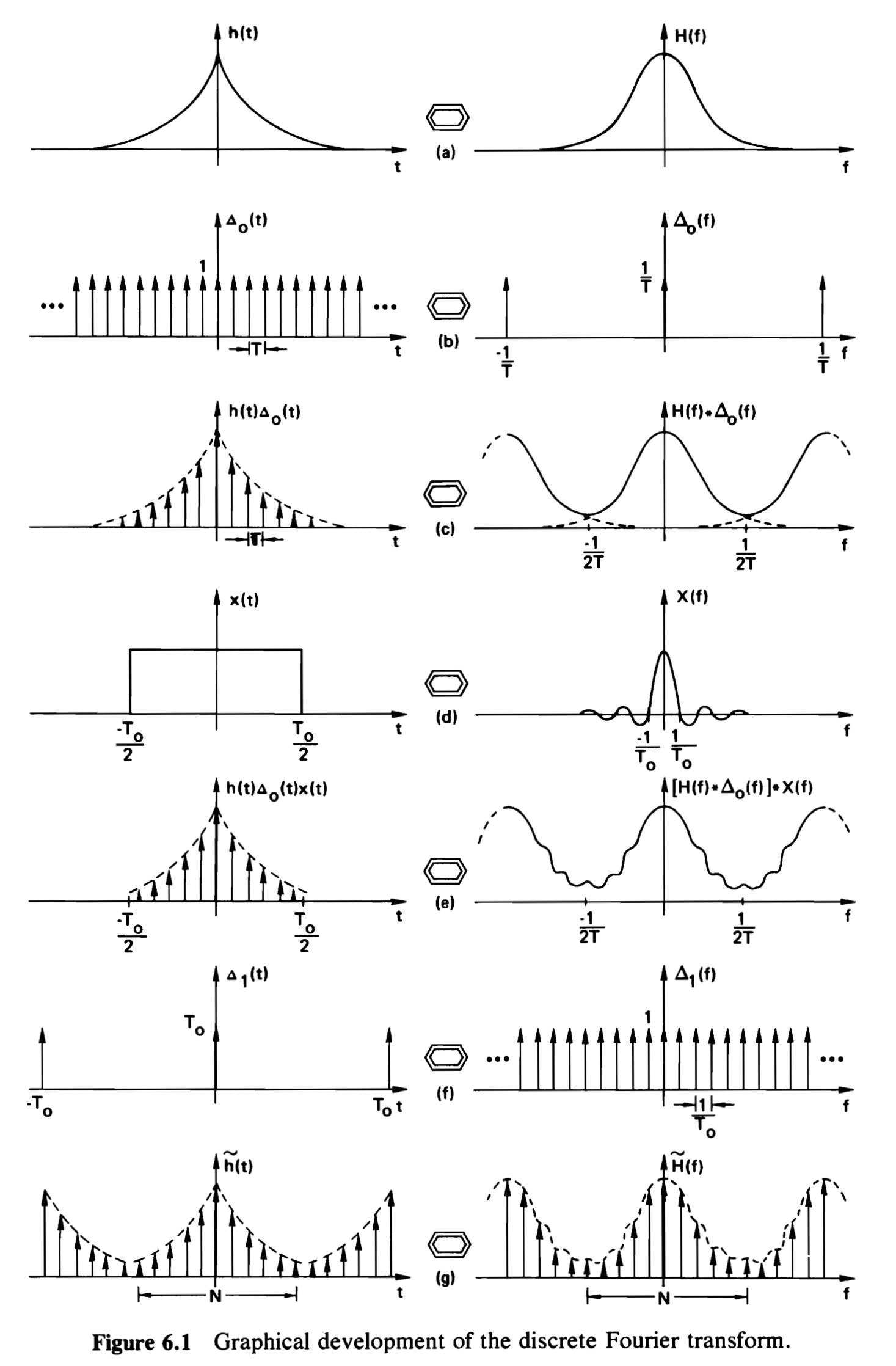
The formulaic derivation as the start of this section is illustrated nicely in Figure 21 from Brigham (1988). The steps are:
Start with \(h\) (our \(F\)) on the left and its ft \(H\) (our \(\hat F\)) on the right.
Sample using the shah-function, a sequence of impulses, Section 4.9. This function is self-dual.
The third step is the product of the first two.
Truncate by multiplying by a rectangular function on the left.
Product of c and d.
Sample on the ft side.
Product of e and f.
Figure 21: Graphical development of the discrete Fourier transform (Brigham 1988)
4.6 Simpson’s Rule
The accuracy of the FFT method can be improved by using Simpson’s rule in the Riemann sum approximations, an idea suggested by Wang and Zhang (2008). This is useful for the stable distribution, where the approximation can be poor in the tails, see the examples in Section 3.6. To start, assume \(x_{\min{}}=0\). Recall \(P=nb\) and the maximum sampling frequency is \(1/b\). The standard approach uses the simplest approximation to the integral \[
f(kb) = \int_{-\infty}^{\infty}e^{2\pi i kb t}\hat f(t)\,dt
\approx \frac{1}{P}\sum_{l=-n/2}^{n/2-1} e^{2\pi i kl/n}\hat f(l/P).
\] The sum is then computed as the IFFT of the vector \((\hat f(l/P))_l\). This approximation corresponds to taking the left-hand value in each sub-interval of the Riemann sum. Equally, we could take the right-hand value, or average the two (trapezoid rule). Or, we could use Simpson’s rule that averages the left, middle, and right values, estimating \[
\int_a^b f(x)\,dx \approx \frac{b-a}{6}(f(a) + 4f((a+b)/2) + f(b)).
\] This can be used in the derivation, after making adjustments both before and after taking the IFFT. In the general case, where \(x_{\min{}}\not=0\), we are trying to calculate for \(k=0,\dots, n\)\[
\begin{aligned}
f_h(x_{\min{}} + kb)
&\approx \frac{1}{P}\sum_{l=-n/2}^{n/2-1} e^{2\pi i (x_{\min{}} + kb)(l+h)/nb}\hat f(l/P) \\
&= e^{2\pi i x_{\min{}}h/P} e^{2\pi i kh/n} \frac{1}{P} \sum_{l=-n/2}^{n/2-1} e^{2\pi i kl/n} \left(e^{2\pi i x_{\min{}}l/P}\cdot \hat f(l/P)\right) \\
&=e^{2\pi i x_{\min{}}h/P} \left(e^{2\pi i kh/n} \cdot \mathrm{IFFT}\left(e^{2\pi i x_{\min{}}l/P}\cdot \hat f(l/P)\right)\right)
\end{aligned}
\] with \(h=0,1/2, 1\) corresponding to left, middle, and right hand Simpson’s terms. In the last row, the first term on the right only depends on \(h\). The next term is a component-by-component product of vectors depending on \(k\). Likewise, the argument to IFFT is a component-by-component product of vectors indexed by \(l\). The three estimates \(f_0, f_{1/2}, f_1\) are then weighted down as vectors \[
f_s \approx \frac{1}{6}(f_0 + f_{1/2} + f_1)
\] to obtain the Simpson inverse approximation. Using Simpson’s rule produces materially estimates for the stable, as Figure 22 shows.
(b) Comparison of basic and Simpson method density, showing considerable improvement in the tails. The orange exact p line is limited by the numerical implementation on the right.
Figure 22: Stable distribution example using Simpson’s rule method.
4.7 Dirac delta functions
This subsection and the remainder of this section provides more general background on fts.
It is helpful to have a “function” with the properties \[
\begin{gathered}
\delta(t-t_0) = 0,\ \forall t\not=t_0 \phantom{\int} \\
\int_{-\infty}^{\infty} \delta(t-t_0)\,dt = 1.
\end{gathered}
\] Such functions emerge as limits. They are called impulse or delta functions. Papoulis (1962) discusses two other properties: they can be a limit of functions satisfying \[
\int_{-\infty}^{\infty} f_n(t)\,dt=1 \quad
\lim_{n\to\infty} f_n(t) = 0 \ \ \forall t\not=0,
\] or have the property that \[
\int_{-\infty}^{\infty} \delta(t)\phi(t)\,dt= \phi(0).
\]
The delta function \(\delta(t)\) is a so-called distribution assigning to the test function \(\phi(t)\) the number \(\phi(0)\). Test functions can be continuous with finite support and continuous derivatives of all order. \(\delta\) defines a continuous linear functional on the set of test functions that is sometimes written using inner-product notation \[
(\delta, \phi) = \int_{-\infty}^{\infty} \delta(t)\phi(t)\,dt = \phi(t).
\] Because of the range of the integral, we can change variables to see \[
\int_{-\infty}^{\infty} \delta(t-t_0)\phi(t)\,dt = \int_{-\infty}^{\infty}\delta(s)\phi(s+t_0)\,ds = \phi(t_0)
\] which Brigham calls the sifting property, as in sifting out a single value—not shifting! Similarly \[
\delta (at) = \frac{1}{|a|}\delta (t).
\] The product of \(\delta\) and a function \(h\) continuous at \(t=t_0\) is \[
(\delta h, \phi) = (\delta, h\phi).
\] You have problems with the associativity: \[
\left( \frac{1}{x} x \right)\delta = \delta
\] but \[
\frac{1}{x} (x\delta) = \frac{1}{x} 0 = 0.
\](Terras 2013, p. 6). The convolution is \[
\delta_1(t-t_1) \star \delta_2(t - t_2) = \delta(t - (t_1 + t_2)).
\]
Given a sequence \(g_n\) of distributions, if there is a distribution \(g\) so that for all test functions \(\phi\)\[
\lim_{n\to\infty} \int_{-\infty}^{\infty} g_n(t)\phi(t)\,dt
= \int_{-\infty}^{\infty} g(t)\phi(t)\,dt
\] then say \[
g(t) = \lim_{n\to\infty} g_n(t).
\] Likewise with ordinary functions \(f_n\), if \[
\lim_{n\to\infty} \int_{-\infty}^{\infty} f_n(t)\phi(t)\,dt = \phi(0)
\] for all test functions, then \[
\delta(t) = \lim_{n\to\infty} f_n(t).
\]
The Riemann-Lebegue lemma says that if \(\phi\) is absolutely integrable on \((a,b)\), where \(a,b\) are finite or infinite constants, then \[
\lim_{\omega\to\infty} \int_a^b e^{-2\pi i\omega t} \phi(t)\,dt = 0.
\]
(Papoulis 1962 Eq I.47) shows \[
\delta(t) = \lim_{\omega\to\infty}\frac{\sin\omega t}{\pi t}.
\] To see this, it suffices to show \[
\lim_{\omega\to\infty} \int_{-\infty}^{\infty} \frac{\sin\omega t}{\pi t}\,\phi(t)\,dt = \phi(0)
\tag{6}\] for continuous, bounded variation \(\phi\). Split the integral into three, the middle one an interval \((-\epsilon, \epsilon)\) around \(0\). The left and right parts are zero by Riemann-Lebesgue. In the middle interval \(\phi(t)\approx \phi(0)\) provided \(\epsilon\) is small enough. Then \[
\int_{-\epsilon}^{\epsilon}\frac{\sin\omega t}{\pi t}\,\phi(t)\,dt
\approx \phi(0) \int_{-\epsilon}^{\epsilon}\frac{\sin\omega t}{\pi t}\,dt
\approx \phi(0) \int_{-\epsilon\omega}^{\epsilon\omega}\frac{\sin t}{\pi t}\,dt
\] (note that \(dt/t\) is scale invariant Haar-measure on \(\mathbb R^\times\)). Since \[
\int_{-\infty}^\infty \frac{\sin x}{\pi x}\, dx = 1
\tag{7}\] the result follows. This integral is an application of contour integration applied to \(e^z/z\) along a half annulus sliced vertically that skirts round the origin, (Papoulis 1962 , II.57).
The highly suspect looking result \[
\int_{-\infty}^\infty \cos\omega t\,d\omega = 2\pi\delta(t)
\] can be interpreted to sensibly if the LHS is regarded as \[
\lim_{W\to\infty}\int_{-W}^{W} \cos \omega t\, d\omega
=\lim_{W\to\infty} \frac{2\sin Rt}{t}
=2\pi\delta(t).
\]
4.8 Approximate identities
Grafakos (2024) Section 1.9 describes that the “futile search” for \(f_0\in L^1(\mathbb R)\) so that \(f_0 * f= f\) for all \(f\in L^1(\mathbb R)\) leads to the notion of approximate identities, a family of functions \(K_\delta\) on \(\mathbb R\) so that:
\(\forall \gamma>0: \int_{|y|>\gamma} K_\delta(y)\,dy=1\) as \(\delta\to 0\).
If \(K\) is integrable with integral \(1\) then \(K_\delta(x) = K(x/\delta) / \delta\) is an approximate identity. \(K(x)=(\pi(x^2+1))^{-1}\) is the Poisson kernel. For an approximate identity, \(K_\delta * f\to f\) as \(\delta\to 0\) in \(L^p\), \(1\le p<\infty\), and if, in addition, \(f\) is uniformly continuous in a neighborhood of \()\) then this is also true for \(p=\infty\). The proof of this is a bit of work and is key to Fourier inversion. It uses the approximate identity \[
K_\delta(x) = \frac{1}{\delta} e^{-\pi \delta^2 x^2}.
\]
The shah or sampling function is defined as \[
\text{ш}_b(t) = \sum_k \delta(t - kb).
\] It is like an equally likely selection from the integers! Terras (2013) says the name reflects the graph, a series of spikes. It can be understood from Figure 23, which shows convergents of the sum \[
f(t) = \sum_{k=-n}{n} \cos(2\pi kt)
\] for \(n=1,\dots,6\). Each term adds two \(\delta\) functions, per Equation 8.
The ft of \(f(x)=\cos(2\pi\omega x)\) is \((\delta(t-1) + \delta(t+1))/2\) because \[
\begin{aligned}
\hat f(t)
&= \int_{-\infty}^{\infty}e^{-2\pi i xt}\cos(2\pi\omega x)\,dx \\
&= \frac{1}{2}\int_{-\infty}^{\infty}e^{-2\pi i xt}(e^{2\pi i \omega x}+e^{-2\pi i \omega x}))\,dx \\
&= \frac{1}{2}\int_{-\infty}^{\infty}e^{-2\pi i x(t-\omega)} + e^{-2\pi i x(t + \omega)}\,dx \\
&= \frac{1}{2}\int_{-\infty}^{\infty}\cos(2\pi x(t-\omega)) + \cos(2\pi x(t+\omega))\,dx \\
&= \frac{1}{2}\left( \frac{\sin(2\pi x(t-\omega))}{2\pi (t-\omega)}\bigg\vert_{-\infty}^{\infty} + \frac{\sin(2\pi x(t+\omega))}{2\pi (t+\omega)}\bigg\vert_{-\infty}^{\infty} \right) \\
&= \frac{1}{2}\left( \lim_{R\to\infty} \frac{\sin(2\pi R(t-\omega))}{\pi (t-\omega)} + \lim_{R\to\infty}\frac{\sin(2\pi R(t+\omega))}{\pi (t+\omega)} \right) \\
&=\frac{1}{2}\left( \delta(t-\omega) + \delta(t+\omega) \right)
\end{aligned}
\tag{8}\] using the fact that the function \(\cos{}\) is even and \(\sin{}\) is odd.
The ft of ш is \[
\hat{\text{ш}}_b = \sum_k \hat \delta(t - kb) = \frac{1}{b} \text{ш}_{1/b}
\]
Multiplying a distribution by \(\text{ш}\) creates sampled distribution: \[
f_b(t) = f(t) \times \text{ш}_b(t) = \sum_k p_k\delta(t-kb).
\] The sampled distribution has ft \[
\hat{f_b} = \widehat{f \text{ш}_b} = \hat f \hat{\text{ш}}_b
= \frac{1}{b} \hat f \text{ш}_{1/b}.
\] Compare, second discretizing steps in Section 4.5.
4.10 Code
The code for FourierTools.invert is shown below. It reveals how the arguments are selected when not passed explicitly. It is designed for loss distributions that usually start at \(0\). The variable self refers to an object that knows the ch f and has a variable fz providing the standard probability functions.
The effective range of \(X\) is \(x_\mathrm{range}= x_{\max{}}-x_{\min{}}\). The discretization bucket size is \[
b = \frac{x_\mathrm{range}}{n} = \frac{x_{\max{}}-x_{\min{}}}{n}.
\tag{9}\] The highest sampled frequency is \[
f_{\max{}} = \frac{1}{b}
\] since wavelength is the reciprocal of frequency (if you sample every 1/4 step, then you sample four times per step). If \(X\) is discrete and takes integer values, it is best to require that \(x_{\min{}}\) and \(x_{\max{}}\) are integers and \(x_{\max{}} = x_{\min{}} + n\), resulting in \(b=1\). It is usually preferable to input bs and let x_max fallout.
def invert(self, log2, x_min=0, bs=0, x_max=None, s=1e-17):# number of bucketsself.log2 = log2 n =1<< log2if x_min isNone:# use quantile function if not given x_min x_min =self.fz.ppf(s)if bs ==0:ifself.discrete:# force bs = 1 x_max = x_min + nelse:# use quantile function is not given x_max x_max =self.fz.isf(s) if x_max isNoneelse x_maxelse: x_max = x_min + bs * n x_range = x_max - x_min# discretization step bs = x_range / n# highest sampling freq for inverting the FT is 1 / bs f_max =1/ bs# sample the FT; using real fft, only need half the rangeself._ts = np.linspace(0, 1/2, n //2+1) * f_max# apply ftself._fourier =self.fourier_transform(self._ts)# invert using real IFFT routine probs = irfft(self._fourier)# roll back to put x_min in the correct spotif x_min !=0: probs = np.roll(probs, -int(x_min / bs))# add index of implied x values df = pd.DataFrame({'x': np.linspace(x_min, x_max, n, endpoint=False),'p': probs}).set_index('x')return df
5 More Examples
Because I find Fourier techniques so magical I can’t resist giving more examples. The new lessons are only that the scipy.special implementation of \({}_1F_1\) is very poor and that fts don’t like discontinuities, see the uniform example, Section 5.5. Otherwise, they all confirm the relationship between the ch f for each distribution and its scipy.stats implementation, and that the algorithm in Section 1 works!
5.1 Binomial
The binomial has two shape parameters.
Code
n, p =64, .25fz = ss.binom(n, p)log2 =7ft_obj = FourierTools( chf=lambda t: (1- p + p * np.exp(1j* t)) ** n, fz=fz )ft_obj.invert(log2=log2, x_min=0, x_max=0)# print(ft_obj.describe())ft_obj.compute_exact(calc='survival')ft_obj.plot()
Figure 24: Binomial distribution example.
5.2 Normal
The normal has no shape parameters. Scale and location are handled automatically by adjusting the ft.
Figure 28: Gamma distribution with shape equal \(100\) centered by shifted left by \(100\).
5.3.4 Gamma with bad aliasing
This example uses an interval \(I=[0,P)\) that is too small to contain the bulk of the support. The problem is that \(P=nb\) is too small; this is even a problem if \(n\) is very large (with \(b\) correspondingly small). The top left plot in Figure 29 show aliasing across the entire range; Figure 30 shows it is largely accounted for by the two translated \([P,2P)\) and \([2P,3P)\).
Figure 32, top left, shows the ft doesn’t like discontinuities. The overshoot is known as Gibbs Phenomenon. It is an unavoidable problem, reflecting the difficulty of approximating a discontinuous function with a series of continuous functions. Note the \(y\) axis scale in the first plot!
Figure 32: Inversion of a uniform distribution with Gibbs ringing in the second plot.
5.6 Beta
The beta distribution turns out to be tricky because there was an error in \(_1F_1\) in scipy see Issue #20797. It was fixed in a later release, however, even after fix the new version is not that accurate for complex arguments. To avoid jumps we work with the beta shown in Figure 33, using parameters \(a=5\) and \(b=12\).
Figure 33: Beta density with no jumps at domain endpoints.
The mpmath implementation of the hypergeometric function that is needed for the beta ch f turns out to be more reliable than the scipy.special’s.
Code
from mpmath import hyp1f1def beta_chf(a, b, t):"""Compute beta chf at t. Includes the 1j factor."""ifisinstance(t, (float, int)):returncomplex(hyp1f1(a, a + b, 1j* t))else:return np.array([complex(hyp1f1(a, a + b, 1j* z)) for z in t])
Brigham, E. O. (1988). The fast fourier transform and its applications. Prentice Hall.
Grafakos, L. (2008). Classical fourier analysis (2nd ed.). Springer.
Grafakos, L. (2009). Modern fourier analysis. Springer.
Grafakos, L. (2024). Fundamentals of fourier analysis. Springer.
Hewitt, E., & Ross, K. A. (2012). Abstract harmonic analysis: Volume i: Structure of topological groups integration theory group representations (Vol. 115). Springer Science & Business Media.
Jørgensen, B. (1987). Exponential Dispersion Models. Journal of the Royal Statistical Society Series B, 49(2), 127–162.
Körner, T. W. (2022). Fourier analysis. Cambridge university press.
McCullagh, P., & Nelder, J. A. (2019). Generalized linear models. Routledge.
McKean, H. (2014). Probability: The classical limit theorems. Cambridge University Press.
Mildenhall, S. (2024). Aggregate: fast, accurate, and flexible approximation of compound probability distributions. Annals of Actuarial Science, 1–40. https://doi.org/10.1017/S1748499524000216
Mittnik, S., Doganoglu, T., & Chenyao, D. (1999). Computing the Probability Density Function of the Stable Paretian Distribution. Mathematical and Computer Modelling, 29, 235–240.
Nolan, J. P. (2020). Univariate stable distributions. Springer Series in Operations Research and Financial Engineering, 10, 978–3.
Papoulis, A. (1962). The fourier integral and its applications. McGraw-Hill, New York.
Terras, A. (2013). Harmonic analysis on symmetric spaces—euclidean space, the sphere, and the poincare upper half-plane. Springer Science & Business Media.
Wang, L., & Zhang, J.-H. (2008). Simpson’s rule based FFT method to compute densities of stable distribution. In The second international symposium on optimization and systems biology (pp. 381–388). Lijang, China.
Source Code
---title: Inverting Characteristic Functions Using FFTsdate: '2025-01-23'date-modified: last-modifieddescription: How to use FFTs to invert the characteristic function of a probability distribution.categories: - notesdraft: falseimage: img/banner.pngauthor: - name: Stephen J. Mildenhall orcid: 0000-0001-6956-0098 corresponding: true email: mynl@me.comcolorlinks: truelink-citations: truelink-bibliography: truetbl-align: centernumber-sections: truecode-line-numbers: false # html and pdfcode-overflow: wrap # html only ,pdf already wrapscode-fold: true # html only fold buttoncode-copy: true # html only copy button in blockcode-tools: true # html only tools buttonformat: html: smooth-scroll: true citations-hover: true crossrefs-hover: false footnotes-hover: true link-external-icon: true link-external-newwindow: true page-layout: article fig-responsive: true lightbox: true ft_obj-contained: false reference-section-title: ' ' css: - algo.css fig-format: svg fig-align: left toc: true toc-depth: 3 toc-title: 'In this post:' pdf: documentclass: article papersize: a4 fontsize: 12pt keep-tex: true geometry: margin=1in fig-format: pdf fig-align: left # fig-dpi: 600 pdf-engine: lualatex pdf-engine-opts: - '-interaction=nonstopmode'bibliography: - books.bib - library.bibcsl: style.cslexecute: eval: true echo: true error: true cache: true cache-type: jupyter freeze: false kernel: python3 engine: jupyter daemon: 1200jupyter: jupytext: text_representation: extension: .qmd format_name: quarto format_version: '1.0' jupytext_version: 1.16.4 kernelspec: display_name: Python 3 (ipykernel) language: python name: python3---```{python}#| echo: false#| label: invisible-spacer# just separate header from first text blobpass# %run -m great2.startup```{width=50%}# Introduction {.unnumbered}This post describes how to use FFTs to invert the characteristic function (ch f) of a probability distribution to recover the underlying distribution. This is a valuable technique for distributions such as the stable and Tweedie that have a closed form characteristic function but not probability density or cumulative probability funciton. It is also instructive to see how Fourier transforms and characteristic functions relate to FFTs.The post is in five sections. @sec-algo describes the algorithm and @sec-errors describes the errors it may be introduce. @sec-core-examples provides eight core examples, illustrating different behaviors and shows how to use the [`unwrap`](https://aggregate.readthedocs.io/en/latest/3_reference/3_x_Distribution.html#aggregate.distributions.Aggregate.unwrap) function recently added to [`aggregate`](https://aggregate.readthedocs.io/en/latest/). @sec-background lays out the background and theory in more depth. @sec-more-examples adds more examples.*Abbreviations.* Throughout the post: ch f is characteristic function, pdf and cdf the probability density and cumulative density function, ft (ift) the (inverse) Fourier transform, and FFT (IFFT) the (inverse) Fast Fourier Transform.# Algorithm {.mt-3 #sec-algo}To invert a ch f using the FFT you must determine the effective support interval of the distribution, convert the ch f into a Fourier transform and sample it, invert the sample using the FFT, and finally translate the result to the desired support interval. Here are the details of the algorithm. @sec-sampling explains why it works.<div class="algorithm lst-main mb-3">### Algorithm to Invert a Characteristic Function Using FFTs {.unnumbered .mt-1}<div class='mt-1'></div>1. **Inputs.** 1. The characteristic function $\phi(t)$ of a distribution $F$. 2. An interval $I=[x_{\min{}}, x_{\max{}}]\subset\mathbb R$ with $F(x_{\max{}})-F(x_{\min{}})$ close to $1$. 3. The number of samples $n=2^{\log_2}$ for an integer $\log_2\ge 1$.<div class='mt-1'></div>2. **Computations.** 1. $b = x_\mathrm{range}/ n = (x_{\max{}}-x_{\min{}})/n$, the discretization step size. 2. $f_{\max{}} = 1 / b$, the maximum sampling frequency. 3. Sample the Fourier transform $\hat F(t)=\phi(-2\pi t)$ at the points $t_l = l f_{\max{}} / n$ for $l=0,1,\dots,n/2+1$ to obtain a vector $\mathsf v = (\hat F(t_l))_l$. 4. Take the real IFFT of $\mathsf v$ to obtain a vector $\mathsf p=(p_0,\dots,p_{n-1})$.<div class='mt-1'></div>3. **Results.** For $k=0,\dots,n-1$ $$ p_k \approx \sum_{m\in \mathbb Z} F((mn + k + 1/2)b) - F((mn + k - 1/2)b). $$ {#eq-aliasing-error}</div>When condition (1.2) holds we say informally that $I$ contains the **effective support** of $X$.The $p_k$ in @eq-aliasing-error are periodic, with period $n$. The condition in step (1.2) means that the effective support is contained in one period. The only trick is to match $k$ to the desired $x$-scale. For that, it is best to select $x_{\min{}}$ as an integer multiple of $b$ (automatically true when $x_{\min{}}=0$), say $x_{\min{}} = m_0b$. Then$$\begin{aligned}\Pr(X\in (x_{\min{}} &+ (k-1/2)b, x_{\min{}} + (k-1/2)b]) \\&= F((m_0 + k + 1/2)b) - F((m_0 + k - 1/2)b) \\&\approx p_k.\end{aligned}$$In turn$$F((m_0 + k + 1/2)b) - F((m_0 + k - 1/2)b) \approx f(m_0 + kb)b$$ {#eq-disc-error}provided $b$ is small enough, which gives an estimate of the density if it exists. The rationale behind these steps is laid out in @sec-background.The value $x_{\min{}}$ is often known from the support of $X$. For example, it is $0$ for any non-negative $X$ such as the standard lognormal or gamma.If $F$ can be computed, the inputs $x_{\min{}}$ and $x_{\max{}}$ can be determined as quantiles $q(s)$ and $q(1-s)$ of $F$ for small $s$.*Philosophical aside.* There is a chicken-and-egg problem here: how to determine $I$ if $\phi$ is known but not $F$? $I$ can be input based on an inspired guess. If it is not given, the routine `FourierTools.invert` cheats by requiring $F$ is given and then determines $I$ using lower and upper quantiles. If you really don't know $F$, then determine the maximum sampling frequency $f$ so that $|\phi(-2\pi f)|$ is very small (a ft always tends to zero as $f\to\infty$). The inverse of the sampling frequency is a good choice for the discretization step size $b=1/f$. Then, determine $n$ so that $nb$ is large enough to contain all the features of the distribution, through a process of trial an error if necessary. In practice, you always know enough about $F$ to estimate quantiles.# Errors {.mt-3 #sec-errors}There are three sources of error in the FFT algorithm of @sec-algo.1. **Aliasing error** whereby the tail of $X$ wraps around into $I$, @eq-aliasing-error. We want $p_k=F((k+1/2)b)-F(k-1/2)b)$ but end up with $\sum_{m\in\mathbb Z} F((mn + k +1/2)b)-F(mn + k - 1/2)b)$. Aliasing is controlled by ensuring $I$ is long enough to be the effective support, containing the preponderance of the probability. Since $I$ has length $P=nb$, once $b$ is selected aliasing is controlled by making $n$ large enough.1. **Discretization error** results from replacing the original distribution with a discretized approximation, @eq-disc-error. It is controlled by decreasing the bucket size $b$. The error comes from the difference between $f(kb)b$ and $F((k+1/2)b)-F(k-1/2)b)$. It manifests as a smearing of details: narrow spikes in $F$ are lost. There is no discretization error for a discrete distribution when $b=1$.1. **Truncation error** results from replacing $\int_{-\infty}^\infty$ with $\int_{-f_{\max{}}}^{f_{\max{}}}$ when the ft is inverted, because the algorithm uses a finite sample. Truncation error is rarely an issue because ft functions typically tend to zero quite quickly. Since $f_{\max{}}=1/b$, truncation error normally occurs in conjunction with discretization error ($b$ too large, $f_{\max{}}$ too small). However, it manifests differently, as negative probabilities| Type of Error | Manifestation | Cause | Examples ||:---------------|:----------------------------|:------------------|:---------|| Aliasing | Tails wrap around into body | $nb$ too small | @sec-po-alias, @sec-po-extreme-alias, @sec-stable || Discretization | Fine detail of $F$ lost | $b$ too large | || Truncation | Negative probabilities | $f=1/b$ too small | @sec-gamma-trunc |: Manifestation and cause of errors and corresponding examples. {#tbl-errors .tbl-colwidth="20% 30% 10% 40%"}# Core examples {.mt-3 #sec-core-examples}## Python set up {.unnumbered}Here is the Python code needed to run examples. The code relies on an up to date version of the [`aggregate` package](https://aggregate.readthedocs.io/en/latest/index.html), available from [GitHub](https://github.com/mynl/aggregate) and [PyPi](https://pypi.org/project/aggregate/). This is standard programming nonsense.```{python}#| label: setup#| echo: true#| code-fold: showfrom aggregate import __version__ as vif v <'0.24.2':raiseValueError('Need aggregate v0.24.2 or later.\n''Run pip install -U aggregate to update.')from aggregate import buildfrom aggregate.extensions.ft import FourierTools, make_levy_chfimport scipy.stats as ssimport numpy as npimport pandas as pdimport matplotlib.pyplot as pltfrom IPython.display import displaydef my_ff(x):"""My float formatter."""try:if x ==int(x):returnf'{x:,d}'elifabs(x) <0.005:returnf'{x:.5g}'elifabs(x) <100:returnf'{x:.3f}'else:returnf'{x:,.0f}'except:returnstr(x)pd.options.display.float_format = my_fftry:from greater_tables import qdexceptModuleNotFoundError:print('Greater tables not found...using IPython.display.') qd = display# qd = display```## Basic example, Poisson distribution {#sec-po-basic}The first example uses a Poisson with mean 10. The bucket size $b=1$ because the Poisson is discrete, and $n=2^5=32$ buckets, providing enough "space" to capture the full range of outcomes. There is no discretization error (already discrete) and imperceptible aliasing since $\Pr(N>32)=7.37\times 10^{-9}$. The distribution starts at $x_{\min{}}=0$. The ch f of a Poisson with mean $n$ is$$\phi(t) = e^{n(e^{it}-1)},$$see [Poisson distribution on Wikipedia](https://en.wikipedia.org/wiki/Poisson_distribution). Throughout the post, ch f's are taken from Wikipedia.This, and all subsequent code blocks follows the same pattern. Create the `FourierTools` object, passing in the ch f and a `scipy.stats` distribution. The latter is used to estimate the effective support and plot the numerical results against the actual. The object method `invert` does the work, the code is shown [below](#code). The `plot` method produces the graphic.```{python}#| label: fig-po-basic#| fig-cap: Poisson, mean 10.#| echo: trueen =10ft_obj = FourierTools( chf=lambda t: np.exp(en * (np.exp(1j* t) -1)), fz=ss.poisson(en))ft_obj.invert(log2=5, x_min=0)# print(ft_obj.describe())ft_obj.compute_exact()print(f'Pr(Po(10)>=32) = {ft_obj.fz.sf(32):.4f}')ft_obj.plot()```The six plots in @fig-po-basic show, clockwise from top left:1. The density created by Fourier inversion (solid blue) and the true density per `scipy.stats` (dashed red).2. Density on a log scale, to show possible differences in the tail more starkly. Here they agree over the entire range.3. The survival and cumulative distribution functions $\Pr(X>x)$ and $\Pr(X\le x)$ respectively. The cdf is in blue and red, sf in green and purple; solid Fourier, dashed exact.4. The sampled Fourier transform. The blue line shows the actual transform, which usually decreases quickly to $0$. The orange line shows $\hat F / |\hat F|$ to show how the ft wraps around the origin.5. The amplitude (purple line, left log-scale) and phase (green, right scale) of the ft. The unwrapped phase tries to correct for the ft wrapping around the origin using `np.unwrap`.6. The log survival and cumulative distribution functions. A log version of the plot above it to make tail behavior more obvious.::: {.callout-note}The first four examples use a Poisson distribution for simplicity, but could equally use any other continuous distribution.:::## Poisson with aliasing {#sec-po-alias}Here is a simple example of aliasing (wrapping), using the same Poisson with mean of $10$ but only $n=2^4=16$ buckets. This is not enough space to contain the answer, and the right tail of the distribution wraps around and appears on the left as the uptick in the blue line in the first and second plots.```{python}#| label: fig-po-alias-1#| fig-cap: Poisson, mean 10 with too few buckets introducing aliasing.ft_obj.invert(log2=4, x_min=0)# need to recompute because wraps works off actualft_obj.compute_exact(calc='survival')print(f'Pr(Po(10)>=16) = {ft_obj.fz.sf(16):.4f}')ft_obj.plot()```@fig-po-alias-2 decomposes the aliasing. Clockwise from the top left:1. The Fourier result (blue), the exact result (red dashed) and the tail that wraps around (thin green).2. As first plot, but showing each result incrementally, and showing the tails in context. The vertical lines mark off the periods of width $nb=P$. The small gaps between the wrap segments have width $b$. They are visible only when $b$ is large relative to $n$, as in this case where $b=1$ and $n=16$.3. Plot 2 on a log $y$ scale, making it clear how the wraps are translated left into the first column.4. Plot 1 on a lot $Y$ scale.The second plot makes the source of the aliasing clear.```{python}#| label: fig-po-alias-2#| fig-cap: Aliasing, showing how different translates wrap-around.df = ft_obj.plot_wraps([1, 2], add_tail=True)ft_obj.last_fig.axes[1].legend().set(visible=False);```## Poisson with extreme aliasing {#sec-po-extreme-alias}@fig-po-extreme-1 illustrates more extreme aliasing. It shows an attempt to model a compound Poisson distribution with a mean of $256$ using only $32$ buckets. The standard deviation is 16, and a normal approximation indicates the width of $I$ should be at least $6\times 16= 96$ (for $\pm 3\sigma$). The result is the almost straight blue line, top left. The remaining plots are largely meaningless.```{python}#| label: fig-po-extreme-1#| fig-cap: Extreme aliasing, Poisson, mean 256, computed with only 32 samples.#| echo: trueen =256ft_obj = FourierTools( chf=lambda t: np.exp(en * (np.exp(1j* t) -1)), fz=ss.poisson(en))ft_obj.invert(log2=5, x_min=0)ft_obj.compute_exact(calc='survival')# print(ft_obj.describe())print(f'99.99%ile of Po(10) is {ft_obj.fz.isf(0.0001)}')ft_obj.plot()```The aliasing plot, @fig-po-extreme-2 top right, explains what is happening. The distribution "lives" between 6 and 9 translations of $I=[0, 32]$ to the right, i.e., between 192 and 320, but is not contained within any single $I$. Each vertical slice is translated back to the origin and added vertically giving the cumulative totals, on the top left.```{python}#| label: fig-po-extreme-2#| fig-cap: Extreme aliasing produces nonsensical results, but the aliasing explains how they occur.df = ft_obj.plot_wraps([6, 7, 8, 9], add_tail=True)ft_obj.last_fig.axes[1].legend().set(visible=False);# for ax in [ft_obj.last_fig.axes[1], ft_obj.last_fig.axes[3]]:# ax.set(xticks=ft_obj.x_min + np.arange(0, 11, 2) * ft_obj.x_max)# ax.xaxis.set_minor_locator(ticker.AutoMinorLocator(n=2))```@tbl-po-extreme-3 shows the probabilities $\Pr(N\in I + kP)$ for $k=6,7,8,9$. None of the slices satisfies the condition in (1.2).```{python}#| label: tbl-po-extreme-3#| tbl-cap: Probabilities in each slice for @fig-po-extreme-2.qd(df)```This example essentially reproduces Figure 1 in @Mildenhall2024.## Poisson with large mean {#sec-large-mean}The case of a Poisson distribution with a very high mean is interesting because it shows that Fourier methods do not need space for the whole distribution, just its effective support. We can use periodicity to translate the answer to the correct outcome range. This example reproduces a Poisson with mean $10,280$. The standard deviation is about $100$ and the effective support of the distribution (using the normal approximation) is about $[9750, 10550]$. Thus, a satisfactory approximation can be obtained with only $2^{10}=1024$ buckets. The second plot shows a very slight aliasing on the left.```{python}#| label: fig-po-large-mean-1#| fig-cap: Poisson, mean 10280, computed using only 1024 buckets by shifting.en =10280ft_obj = FourierTools( chf=lambda t: np.exp(en * (np.exp(1j* t) -1)), fz=ss.poisson(10280))ft_obj.invert(log2=10, x_min=9750)ft_obj.compute_exact(calc='survival')# print(ft_obj.describe())ft_obj.plot()```Adjusting this example to set `x_min=0` shows its effect. @fig-po-large-mean-1 uses $x_{\min{}}=9750$. Setting $x_{\min{}}=0$ results in @fig-po-large-mean-2. It is clear that the density could be sliced vertically and the pieces rearranged to produce the correct density, c.f., @fig-po-extreme-2 top left.```{python}#| label: fig-po-large-mean-2#| fig-cap: Poisson, mean 10280, computed using only 1024 **without** shifting.ft_obj.invert(log2=10, x_min=0)ft_obj.compute_exact(calc='survival')# print(ft_obj.describe())ft_obj.plot()```@fig-po-large-mean-2 essentially reproduces Figure 2 in @Mildenhall2024.## Gamma with frequency-domain truncation error {#sec-gamma-trunc}This example uses too few buckets, resulting in $b$ being too large and $f_{\max{}}$ too small and hence producing discretization error and truncation error. The truncation of the Fourier integral (replacing $\int_{-\infty}^\infty$ with $\int_{-f_{\max{}}}^{f_{\max{}}}$) introduces negative probabilities, @fig-gamma-5 top left and @tbl-gamma-5: there is no way for negative probabilities to occur from aliasing or discretization error. The example uses a gamma distribution with shape $2$.```{python}#| label: fig-gamma-5#| fig-cap: Gamma, shape $\alpha=2$, with only 16 buckets. Truncation error introduces negative probabilities.alpha =2ft_obj = FourierTools( chf=lambda t: (1-1j* t) **-alpha, fz=ss.gamma(alpha, loc=0))ft_obj.invert(log2=4, x_min=0)# print(ft_obj.describe())ft_obj.compute_exact()ft_obj.plot()``````{python}#| label: tbl-gamma-5#| tbl-cap: Negative probabilities caused by truncation of the Fourier integral.qd(ft_obj.df.query('p<0'))```## Stable distributions {#sec-stable}The method described in this post has a practical application approximating members of the important stable family of distributions [@Nolan2020bk], which are otherwise hard to compute in other ways. In fact, the `scipy.stats`[stable class](https://docs.scipy.org/doc/scipy/reference/generated/scipy.stats.levy_stable.html) recently implemented FFT approximations, though these are considered experimental. FFT and other methods of computation are discussed in @Mittnik1999 and @Wang2008a. The latter is implemented and discussed in @sec-simpsons-rule.Stable distributions are determined by two shape parameters: $a\in(0,2)$ and skewness $b\in[-1,1]$. The normal is the limit as $a\to 2$. The skewness has the same sign as $b$, increases with $|b|$, and $b=0$ is symmetric. Two well-known examples are the Cauchy distribution when $a=1$, and the Lévy stable distribution when $a=1/2$ and $b=0$. These are the only cases with a simple pdf or cdf. Stable distributions are all thick tailed with$$\Pr(X>x)\sim \frac{1}{x^{\alpha}},$$meaning smaller $a$ results in thicker tails. If $a \ge 1$ or $b\in (-1,1)$, then the distribution is supported $\mathbb R$. If $a<1$ and $b=-1$ (resp. $b=1$) the support is $(-\infty, 0)$ (resp. $(0, \infty)$). Because of the thick tails, aliasing error is always present to some extent, calling for a large $n$. At the same time, the distributions are quite peaked, calling for a small $b$. They represent a difficult case for FFTs.We can look at the ch f to determine a reasonable bucket size by determining $f$ so $|\hat F(f)|$ is small [@Brigham1988bk chapter 6]. There is no magic way to determine the number of buckets: that requires the quantile function or trial and error. @tbl-stable-1 shows the calculation to estimate $1/b$ for a negatively skewed ($b=-1$) Cauchy.```{python}#| label: tbl-stable-1#| tbl-cap: Determining the bucket size for a negatively skewed Cauchy distribution.a, b =1., -1.levch = make_levy_chf(a, b)# find bs: look for where levch(1/bs) is smalltest = np.arange(0, 11)qd(pd.DataFrame({'b': 1/ test,'1/b': test,'abs ft': np.abs(levch(-2* np.pi * test))} ).set_index('1/b'))```The first example is a negatively skewed Cauchy, $a=1$ and $b=-1$. @tbl-stable-3 shows some quantiles for this thick-tailed, negatively skewed distribution.```{python}#| label: fig-stable-2#| fig-cap: "Cauchy stable distribution with $a=1$ and $b=-1$."a =1.b =-1.fz = ss.levy_stable(a, b)ft_obj = FourierTools( chf=make_levy_chf(a, b), fz=fz )ft_obj.invert(log2=12, x_min=-100, bs=1/32)# print(ft_obj.describe())ft_obj.compute_exact()ft_obj.plot()``````{python}#| label: tbl-stable-3#| tbl-cap: Quantiles for the Cauchy stable distribution with $a=1$ and $b=-1$.# quantilesqd(pd.DataFrame([(p, ft_obj.fz.ppf(p)) for p in [0.001, 0.01, 0.99, 0.999]], columns=['p', 'quantile']).set_index('p'))```@fig-stable-2-large shows the same results with a much wider range of outcomes. The numeric approximation produces non-zero answers only down to about -316.```{python}#| label: fig-stable-2-large#| fig-cap: Cauchy stable distribution with $a=1$ and $b=-1$ with a wider $x$ range.a =1.b =-1.fz = ss.levy_stable(a, b)ft_obj = FourierTools( chf=make_levy_chf(a, b), fz=fz )ft_obj.invert(log2=12, x_min=-1000, bs=0.25)# print(ft_obj.describe())ft_obj.compute_exact()ft_obj.plot()```@fig-stable-4 shows a thinner tailed, positively skewed example.```{python}#| label: fig-stable-4#| fig-cap: Stable distribution with $a=1.75$ and $b=0.3$.a =1.75b =0.3fz = ss.levy_stable(a, b)ft_obj = FourierTools( chf=make_levy_chf(a, b), fz=fz)ft_obj.invert(log2=12, x_min=-50, x_max=100)# print(ft_obj.describe())ft_obj.compute_exact()ft_obj.plot()```@fig-stable-4 shows a thicker tailed, positively skewed example. This example exhibits considerable aliasing to the right because $x_{\min{}}$ is too small. This is decomposed in @fig-stable-6, especially the lower right plot.```{python}#| label: fig-stable-5#| fig-cap: Stable distribution with $a=0.75$ and $b=0.3$.log2 =12a =0.75b =0.3fz = ss.levy_stable(a, b)ft_obj = FourierTools( chf=make_levy_chf(a, b), fz=fz)ft_obj.invert(log2=log2, x_min=-100, x_max=1000)# print(ft_obj.describe())ft_obj.compute_exact()ft_obj.plot()``````{python}#| label: fig-stable-6#| fig-cap: Decomposition of aliasing for @fig-stable-7.ft_obj.plot_wraps([-1, 1,2], add_tail=True);```@fig-stable-7 uses the same distribution with a much tighter range $[-10, 10)$ vs. $[-100, 1000)$. This allows a much smaller $b$ which resolves the shape of the mode at $0$ better, but suffers more aliasing on both sides @fig-stable-8. The aliasing can be partially addressed using Simpson's rule, see @sec-simpsons-rule.```{python}#| label: fig-stable-7#| fig-cap: Stable distribution with $a=0.75$ and $b=0.3$, with small range.a =0.75b =0.3fz = ss.levy_stable(a, b)ft_obj2 = FourierTools( chf=make_levy_chf(a, b), fz=fz)df = ft_obj2.invert(log2=log2, x_min=-10, x_max=10, s=5e-2)print(ft_obj2.describe())ft_obj2.compute_exact()ft_obj2.plot()``````{python}#| label: fig-stable-8#| fig-cap: Decomposition of aliasing for @fig-stable-7.ft_obj2.plot_wraps([-1, 1], add_tail=True);ft_obj2.last_fig.axes[1].legend().set(visible=False);```<!-- # look at difference in bucket size - not interestingax = (ft_obj.df.loc[-5:5].p / ft_obj.bs).plot(drawstyle='steps-mid', lw=.75, label=f'Fourier, b={ft_obj.bs:.3f}')(ft_obj2.df.loc[-5:5].p / ft_obj2.bs).plot(ax=ax, lw=.75, label=f'Fourier, b={ft_obj2.bs:.3f}')b = ft_obj2.df_exact.index[1] - ft_obj2.df_exact.index[0]ft_obj2.df_exact.loc[-5:5].p.plot(ax=ax, lw=.75, label=f'Exact survival, grid={b:.3g}')ft_obj2.compute_exact(calc='density', max_points=1024)b = ft_obj2.df_exact.index[1] - ft_obj2.df_exact.index[0]ft_obj2.df_exact.loc[-5:5].p.plot(ax=ax, lw=.75, label=f'Exact density, grid={b:.3g}')ax.legend()-->## Tweedie with `Aggregate` {#sec-tweedie}This example uses the Tweedie distribution, a Poisson-gamma compound. It is a member of the power-variance function family of exponential distributions and appears commonly as a mixed error distribution in GLM modeling, see @Jorgensen1987 and @Mccullagh2019. First, create a Tweedie from its definition with gamma shape `a=20` and scale `sc=1`, and expected frequency `en=20` as using `aggregate`. The expected mean is 200. The example also illustrates using an `Aggregate` object in place of a `scipy.stats` frozen distribution as the reference. @tbl-tweedie-1 creates the `Aggregate` object and displays distribution statistics.```{python}#| label: tbl-tweedie-1#| tbl-cap: Statistics for Tweedie distribution.#| fold: showa =20.sc =1.en =10fz = build(f'agg Tw {en} claims sev {sc} * gamma {a} poisson')qd(fz.describe.iloc[:, [0,3,6]])```The Tweedie has multiple parameterizations. `aggregate` provides a (horrible, sorry) function `tweedie_convert` to translate between them.```{python}#| label: tbl-tweedie-2#| tbl-cap: Alternative parameterizations of the Tweedie.from aggregate import tweedie_converttc = tweedie_convert(λ=en, α=a, β=sc)qd(tc)````aggregate` also provides a `tweedie` keyword to create an `Aggregate` directly. It takes the parameters mean, $p$, and dispersion ($\sigma^2$) parameters. This version is updated numerically and @tbl-tweedie-2b compares the expected and numerical mean, CV, and skewness, showing a very close match.```{python}#| label: tbl-tweedie-2b#| tbl-cap: Tweedie in `aggregate` using the `tweedie` keyword and alternative parameterization.mu = tc.μp = tc.pdispersion = tc['σ^2']tweedie_agg = build(f'agg TwKW tweedie {mu}{p}{dispersion}')qd(tweedie_agg.describe)```Since `Aggregate` objects have `cdf` and related methods they can be used as frozen objects and passed into `FourierTools`. The manual ch f is easy to derive from those of the Poisson and gamma. @fig-tweedie-3 shows a good match.```{python}#| label: fig-tweedie-3#| fig-cap: "Tweedie distribution, mean 200."tweedie_chf =lambda t: np.exp( en * ((1- sc *1j* t) **-a -1) )ft_obj = FourierTools( chf=tweedie_chf, fz=fz)ft_obj.invert(log2=12, x_min=0, bs=1/4)# print(ft_obj.describe())ft_obj.compute_exact()ft_obj.plot()```Users are sometimes surprised at the form of the Tweedie. As $p\downarrow 1$ it becomes a continuous approximation to a Poisson distribution, except for the mass at zero. This leads to a wildly oscillating density. @fig-tweedie-wild shows the FFT method is up to the task! It also illustrates the use of `FourierTools` without passing a distribution object. In this case, we know from the description of the Tweedie that the mean is $20$ and that the distribution will be close a Poisson with the same mean. That is enough to estimate an appropriate bucket size. The example uses a very small bucket size to capture the details of the density.```{python}#| label: fig-tweedie-wild#| fig-cap: "Tweedie distribution with mean 20 and p close to 1, a continuous approximation to the Poisson—computed with FFTs!"en =20.p =1.001a = (2- p) / (p -1)sc =1/ atweedie_chf =lambda t: np.exp( en * ((1- sc *1j* t) **-a -1) )ft_obj = FourierTools( chf=tweedie_chf, fz=None)ft_obj.invert(log2=16, x_min=0, bs=1/1024)ax = ft_obj.df.p.plot(figsize=(4,2.75), lw=.5, ls='-')```## Compound Poisson with discrete severity {#sec-comp}This section shows how to create a compound Poisson with a discrete severity$$\Pr(X=x_k) = p_k.$$When the expected claim count equals $\lambda$, the compound ch f is given by$$\begin{aligned}\phi(t)&= \mathsf E[e^{it A}]\\&= \mathsf E[\mathsf E[e^{it A} \mid N]]\\&= \mathsf E[\mathsf E[e^{itX}]^N]\\&= \mathsf E[e^{N \log \mathsf E[e^{itX}]}]\\&= M_N(\log(\phi_X(t))) \\&= \exp(\lambda(\phi_X(t)-1)).\end{aligned}$$This formula is implemented as `chf` in the code below.Here is an example with $\lambda = 2$, outcomes $1, 2, 10$ with probabilities $5/8, 1/4, 1/8$. Since all jumps are integers $b=1$ is appropriate. @tbl-discretization-1 shows the compound statistics.```{python}#| label: tbl-discretization-1#| tbl-cap: Discrete severity compound statistics.log2 =7# outcomes and probabilitiesxs = np.array([1, 2, 10])ps = np.array([.625, .25, .125])en =2.# build aggregate objectfz = build(f'agg eg2 {en} claims dsev {xs}{ps} poisson', bs=1, padding=0, log2=log2)# check momentsqd(fz.describe)```@fig-discretization-2 shows the approximation. The distribution is multimodal and it is is fit very precisely over a wide range of outcomes.```{python}#| label: fig-discretization-2#| fig-cap: Discrete aggregate fit well with FFT inversion.def chf(t): sev_phi = ps @ np.exp( 1j* (np.atleast_2d(t) * np.atleast_2d(xs).T))return np.where(t==0, 1., np.exp(en * (sev_phi -1)))ft_obj = FourierTools( chf=chf, fz=fz )ft_obj.discrete =Falseft_obj.invert(log2=log2, x_min=0, x_max=1<<log2)# print(ft_obj.describe())ft_obj.compute_exact()dfe = ft_obj.df_exactft_obj.plot()```## Unwrapping with `Aggregate` {#sec-agg-unwrap}The `Aggregate` class includes an `unwrap` method to shift a compound distribution to the correct location. This is helpful when working with large expected claim counts with a bounded severity. @fig-agg-unwrap-1 illustrates for a compound, Poisson claim count mean $250$ and severity uniform on $1,2,\dots, 11$.The mean is $1500 = 250 \times (1+11)/2$, the CV 7%, and standard deviation about $105$, @tbl-agg-unwrap-2. The distribution is recreated using only $2^9=512$ buckets and $b=1$.Without shifting the pmf (@fig-agg-unwrap-1 left) appears to produce nonsense output. Slicing and rearranging produces the correct output (right).```{python}#| label: fig-agg-unwrap-1#| fig-cap: Unwrapping an aggregate distribution using `Aggregate.unwrap`.en =250apo = build(f'agg PoBig {en} claims dsev[1:11] poisson', bs=1, log2=9, padding=0)fig, axs = plt.subplots(1, 2, figsize=(4.0, 2.0), constrained_layout=True, sharey=True)ax0, ax1 = axs.flatapo.density_df.p_total.plot(ax=ax0, label='aggregate')ax0.set(title='Raw aggregate', xlabel='x', ylabel='pmf')ans = apo.unwrap(p=1e-1)ans.y.plot(ax=ax1)ax1.set(title='Unwrapped aggregate', xlabel='x');``````{python}#| label: tbl-agg-unwrap-2#| tbl-cap: Aggregate distribution statistics.qd(apo.describe)```# Technical Background {.mt-3 #sec-background}## Context and literature> **Complaint.** It is the most natural thing in the world to decompose an oscillating electrical signal into sines and cosines of various frequencies via the Fourier transform - but probabilities, no. Basically, these are positive numbers adding up to 1, and what have sines and cosines to do with that? Indeed, in many applications done first by Fourier, a simpler, more understandable proof may emerge upon taking Fourier away. Still, the Fourier transform is a very effective, sometimes indispensable technical tool in much of our business here. [@McKean2014]>> *Henry P. McKean, Jr. (1930 – 2024) was an American mathematician at the Courant Institute in New York University. He co-authored the famous book "Diffusion processes and their sample paths" with Kioshi Itô.*Fourier transforms and the Fast Fourier Transforms (FFTs) are magic and mysterious and their application to probability is odd (McKean quote) yet extremely effective―providing proofs of the central limit and Lévy-Khinchin theorems and a practical way to add (convolve) distributions, among other uses.There are many treatments of fts and FFTs in the literature. @Brigham1988bk is a very helpful reference providing great diagrams to show what is going on; @sec-ft-cont-disc follows it closely. He develops the continuous and discrete transforms together and explains the connection in Section 6. He refers back to @Papoulis1962bk, who has an interesting appendix on distributions. @Korner2022 is good for historical context and details such as swapping the order of integration. @Terras2013 is good for mathematical context. @Grafakos2008bk provides a modern mathematical view, developed further in @Grafakos2009bk. He has also recently released @Grafakos2024bk. Going hardcore, try @Hewitt2012bk.[@Mildenhall2024](https://www.cambridge.org/core/journals/annals-of-actuarial-science/article/aggregate-fast-accurate-and-flexible-approximation-of-compound-probability-distributions/1BF9A534D944D983B1D780C60885F065) provides technical background on using FFTs to compute aggregate distributions whereas this article mostly focuses on simpler parametric distributions such as the gamma or normal. Figures equivalent to 1 and 2 in the paper are recreated here in @sec-po-extreme-alias and @fig-po-large-mean-2. The [Aggregate help](https://aggregate.readthedocs.io/en/latest/5_technical_guides/5_x_numerical_methods.html#numerical-methods-and-fft-convolution) contains similar examples and more background, again focused on aggregate distributions.*Notation.* We use $b$ for the discretization **b**ucket size, but it is often written $h$ in other references.## Characteristic functions and Fourier transformsThe ch f $\phi$ of random variable $X$ having cdf $F$ is given by$$\phi(t) = \mathsf E[\exp(itX)] = \int_{-\infty}^\infty e^{itx}\,dF(x).$$ {#eq-chf-def}If $X$ is continuous and has a density $f$ this is the same as$$\phi(t) = \int_{-\infty}^\infty e^{itx} f(x)\,dx.$$@eq-chf-def also works when $X$ is discrete or mixed.The ch f is related to the moment generating function $M(t)=\mathsf E[\exp(tx)]=\phi(-it)$. It has the advantage of always existing. The Cauchy distribution, which is thick-tailed on the left and the right, has no MGF.The Fourier transform (ft) of a distribution function $F$ is usually written $\hat F$ and is given by$$\hat F(t)= \int_{-\infty}^\infty e^{-2\pi itx}\,dF(x).$$ {#eq-ft-def}Some authors omit the scaling factor $2\pi$ which introduces constants to the integrals. The ft is related to the ch f by$$\hat F(t) = \phi(-2\pi t).$$The ch f and ft both contain the same information as the distribution function. The inverse transform$$F(t) = \int_{-\infty}^\infty e^{2\pi itx}\hat F(t) \,dt.$$ {#eq-inv-ft}is valid at points where $F$ is continuous.The ft is useful in probability theory because it translates (difficult) convolution into (easy) multiplication.Computing the distribution of a sum of independent random variables (convolution of distributions) is complicated because you have to consider all different ways an outcome can be split.The ft works like exponentiation, which turns (difficult) multiplication into (easy) addition:$$e^a \times e^b = e^{a+b}.$$Likewise, the ft translate convolution of distributions into multiplication of fts.If $X_i$ are independent random variables, $X=X_1+X_2$, and $F_X$ is the distribution of $X$, then$$\hat F_{X_1+X_2}(t) = \hat F_{X_1}(t) \times \hat F_{X_2}(t),$$where the right-hand side is a product of functions. Thus we can convolve as:$$\begin{array}{c c c} X, \ Y & \xrightarrow{+} & X + Y \\ \text{ft} \downarrow & & \uparrow \text{ift} \\ \hat F_{X},\ \hat F_Y & \xrightarrow{\times } & \hat F_{X+Y}.\end{array}$$Of course, this is only useful if it is easy to compute the ft and its inverse—which is where FFTs come in. The FFT is an *extremely quick* way to compute *discrete* fts.## Example Fourier transformDefine$$f(x)=\begin{cases} A & x\in (-x_0, x_0) \\ A/2 & x = -x_0, x_0 \\ 0 & x\not\in [-x_0, x_0]\end{cases}.$$Then$$\begin{aligned}\hat f(t)&= \int_{-\infty}^{\infty} e^{-2\pi i xt} f(x)\,dx \\&= \int_{-x_0}^{x_0} A e^{-2\pi i xt} \,dx \\&= - A \frac{e^{-2\pi i xt}}{-2\pi i t} \bigg\vert_{-x_0}^{x_0} \\&= A \frac{\sin 2\pi t x_0}{\pi t}.\end{aligned}$$The zeros of the ft are at $(1/2x_0)\mathbb Z$ as $x_0$ varies. As $f$ becomes more spread (larger $x_0$) so $\hat f$ becomes more concentrated around $0$.In the simple case $A=1$ and $x_0=a/2\pi$$$\hat f(t) = \frac{\sin a t}{\pi t}.$$These properties are illustrated in @fig-ft-example. Imagining the limit as $x_0\to\infty$ makes it clear that the $\delta$ function (@sec-dirac-delta) and the constant function are transforms. This example is important because $f\in L^1(\mathbb R)$ (is absolutely integrable) but $\hat f$ is not because $|\hat f|$ is not integrable, which shows that the ft is not a mapping from $L^1(\mathbb R)\to L^1(\mathbb R)$.```{python}#| label: fig-ft-example#| fig-cap: "Function (left) and its ft (right). As the function becomes more concentrated (peaked), the ft becomes more diffuse, and vice versa, illustrating the uncertainty principle."fig, axs = plt.subplots(1, 2, figsize=(2*3, 2.25), constrained_layout=True)ax0, ax1 = axs.flatxs = np.linspace(-3, 3, 1001)ts = np.linspace(-5, 5, 1001)for x0 in [1, .5, .25, ][::-1]: A =1 ys = np.where(np.abs(xs) <= x0, A, 0) ax0.plot(xs, ys, lw=1, drawstyle='steps-mid', label=f'width {2* x0}') fty = np.where(ts==0, A *2* x0, A * np.sin(2* np.pi * x0 * ts) / (np.pi * ts)) ax1.plot(ts, fty, label=f'x0 = {x0}', lw=1)ax0.legend()ax1.legend()ax0.set(title='Function: space or outcome', xlabel='$x$', ylabel='$f(x)$')ax1.set(title='Transform: frequency', xlabel='$t$', ylabel='$\\hat f(x)$');```## Continuous, discrete and fast transforms {#sec-ft-cont-disc}There are three things going on when moving from a continuous ft function to discrete FFT:1. Replacing continuous functions with discrete samples by **sampling**.2. **Truncate** limits in the integrals defining the ft to create finite samples.2. Computing the fts using the Fast Fourier transform algorithm.A continuous distribution $F$ can be approximated with a step distribution that takes the constant value $(F((k-1/2)b)-F((k+1/2)b)) / b$ on the interval $[(k-1/2)b)-F((k+1/2)b))$. By Taylor series,$$\frac{F((k-1/2)b)-F((k+1/2)b)}{b} \approx f(kb).$$Here $b$ is the discretization step-size, which we call the bucket size, and $k\in\mathbb Z$.Discrete approximations arise naturally when estimating $F$ from a finite sample, for example.Likewise, a discrete Fourier transform is a discrete approximation to the continuous fts, formed by **sampling** it at evenly spaced points. The DFT is a sequence, rather than a function. It retains the convolution property of fts. For real valued vectors, DFTs are sometimes called discrete cosine transforms (DCT). Sampling can arise from replacing an integral with its Riemann sum approximation.The DFT is a sequence. To be practical a computer, we can only work with finite length vectors, leading to the second step: **truncation**. Truncation comes about by replacing infinite limits in an integral by finite limits. This is justified because the integrand is very small.The finite DFT is the least mysterious things we deal with: it is given by simple matrix multiplication: a $n\times 1$ sample vector is multiplied by the $n\times n$ matrix $(\omega^{ij})_{i,j}$, $\omega=\exp(-2\pi i / n)$, of $n$th roots of unity.Third, it is the **Fast** Fourier transform that makes this a practical approach.The trick with FFTs is *how* they are compute DFTs, exploiting various symmetries in cunning way. The details are explained in many references, but see @Mildenhall2024 for one in an actuarial context.The first two steps are independent of the FFT implementation. General usage can blur the distinction between discrete fts and their computation, and use FFT as a catchall for both.## Sampling: from continuous to discrete transforms {#sec-sampling}This section is key to explaining @sec-algo. We want to create a sample from a distribution by using the FFT to invert a sample of the continuous ft. The samples are all equally spaced, so start by supposing the distribution will be sampled using $n$ buckets of size $b$. How to select $n$ and $b$ is described later. Set $P=nb$. To start, we can evaluate $f(kb)$ using the continuous ift. Let's see what happens if we try to evaluate that continuous integral by discretizing and truncating.$$\begin{aligned}f(kb)&= \int_{-\infty}^{\infty} \,e^{2 \pi i kb t }\hat f(t)\,dt & \text{definition} \\&\approx \frac{1}{P} \sum_{l\in\mathbb Z} e^{2 \pi i kb (l/nb)}\,\hat f(l/P) & \text{discretize, } 1/P \\% &= \frac{1}{P} \sum_{l=-n/2}^{n/2-1} e^{2 \pi i kb lw}\,\hat f(lw) & \text{truncate} \\&\approx \frac{1}{P} \sum_{l=-n/2}^{n/2-1} e^{\frac{2 \pi i}{n} kl}\,\hat f(l/P) & \text{truncate} \\&= \frac{1}{P} \sum_{l=-n/2}^{n/2-1} e^{\tfrac{2\pi i}{n} k l } \int_{-\infty}^{\infty} e^{-2\pi i x(l/P)}f(x)\,dx & \text{definition} \\&\approx \frac{1}{P} \sum_{l=0}^{n-1} e^{\tfrac{2\pi i}{n} k l } b \sum_{j\in\mathbb Z} e^{-2\pi i (jb)(l/nb) } f(jb) & \text{discretize, } b \\&= \frac{1}{n} \sum_{l=0}^{n-1} e^{\tfrac{2\pi i}{n} k l } \sum_{j\in\mathbb Z} e^{-\frac{2\pi i}{n} jl } f(jb) & \text{simplify} \\&= \frac{1}{n} \sum_{j\in\mathbb Z} f(jb) \sum_{l=0}^{n-1} e^{\tfrac{2\pi i }{n} (k-j)l }& \text{rearrange} \\&= \sum_{m\in\mathbb Z} f(kb +mn) & \text{geometric series} \\&= f_P(kb) & \text{periodic version.}\end{aligned}$$The first three lines relate $f(kb)$ to the IFFT (third step). Notice it is just the matrix product of the $n\times n$ matrix $(\omega^{kl})_{k,l}$ and the $n\times 1$ vector $(\hat f(l/P))_l$. Here $\omega=\exp(2\pi i / n)$ is an $n$th root of unity, meaning $\omega^n=1$. The *fast* part converts the matrix product you expect to take of the order of $n^2$ operations into one taking only $n\log_2(n)$. The rest of the derivation figures out what the IFFT actually computes, which turns out to be the periodic version of $f$ (last row) defined by$$f_P(x) = \sum_k f(x + kP).$$If $f$ actually has finite support contained in $[0, P)$, then $f_P=f$. If that is not the case there will be aliasing, a wrapping spill-over of values.The logic of the each step is as follows. The two discretize steps use Riemann sum, with $dx$ equal to $1/P$ and $b$ respectively. The truncate step is justified by $\hat f(t)$ falling off quickly $t\to\infty$. The rearrange step swaps a finite and infinite sum, which is always legitimate (finite sum of lim is lim of sums). The geometric series step uses two properties of roots of unity. First,$$1 + \omega +\cdots + \omega^{n-1} = \frac{1-\omega^n}{1-\omega} = 0.$$Second, if $1 \le l \le n-1$, then $(\omega^l)^n = (\omega^n)^{l} = 1$ and$$\omega^l + \omega^{2l} +\cdots + \omega^{(n-1)l} = \frac{1-\omega^{ln}}{1-\omega} = 0.$$Third, if $l = jn$, then $\omega^l=(\omega^n)^j=1$ and$$1 + \omega^{l} +\cdots + \omega^{(n-1)l} = 1 + \cdots + 1 = n.$$While both the ft and ift are discretized, truncation applies only to the first ift step. The ft wraps and produces aliasing in the penultimate step, which is still over an infinite sum.It is an important fact, known as Poisson's Summation Formula, that $f$ and $f_P$ have the same ft:$$\begin{aligned}\hat f(l/P):&= \int_{-\infty}^{\infty} e^{-2 \pi i x (l/P)}\, f(x)\, dx \\&= \sum_{k\in\mathbb Z} \int_{kP}^{(k+1)P} e^{-2 \pi i x (l/P)}\, f(x)\, dx \\&= \sum_{k\in\mathbb Z} \int_{0}^{P} e^{-2 \pi i (x+kP) (l/P)}\, f(x+kP)\, dx \\&= \int_{0}^{P} e^{-2 \pi i x (l/P)} \sum_{k\in\mathbb Z} f(x+kP)\,dx & \text{!!}\\&= \int_{0}^{P} e^{-2 \pi i x (l/P)}\, f_P(x)\, dx \\&= \hat{f_P}(l/P).\end{aligned}$$The step marked !! requires $kP$ times the argument of $\hat f$, i.e., $l/P$, to be an integer, hence the choice of argument in the first line. It then follows from the Fourier inversion formula for series that$$f_P(x) = \sum_l f(x+lP) = \sum_l e^{2\pi i lx} \hat f_P(l) = \sum_l e^{2\pi i lx} \hat f(l).$$The formulaic derivation as the start of this section is illustrated nicely in @fig-brig-6-1 from @Brigham1988bk. The steps are:a. Start with $h$ (our $F$) on the left and its ft $H$ (our $\hat F$) on the right.b. Sample using the shah-function, a sequence of impulses, @sec-shah. This function is self-dual.c. The third step is the product of the first two.d. Truncate by multiplying by a rectangular function on the left.e. Product of c and d.f. Sample on the ft side.g. Product of e and f.![Graphical development of the discrete Fourier transform [@Brigham1988bk]](img/fc766551b96107c96bc9368cb4cb314e.png){#fig-brig-6-1 width=66%}## Simpson's Rule {#sec-simpsons-rule}The accuracy of the FFT method can be improved by using Simpson's rule in the Riemann sum approximations, an idea suggested by @Wang2008a. This is useful for the stable distribution, where the approximation can be poor in the tails, see the examples in @sec-stable. To start, assume $x_{\min{}}=0$. Recall $P=nb$ and the maximum sampling frequency is $1/b$. The standard approach uses the simplest approximation to the integral$$f(kb) = \int_{-\infty}^{\infty}e^{2\pi i kb t}\hat f(t)\,dt\approx \frac{1}{P}\sum_{l=-n/2}^{n/2-1} e^{2\pi i kl/n}\hat f(l/P).$$The sum is then computed as the IFFT of the vector $(\hat f(l/P))_l$. This approximation corresponds to taking the left-hand value in each sub-interval of the Riemann sum. Equally, we could take the right-hand value, or average the two (trapezoid rule). Or, we could use Simpson's rule that averages the left, middle, and right values, estimating$$\int_a^b f(x)\,dx \approx \frac{b-a}{6}(f(a) + 4f((a+b)/2) + f(b)).$$This can be used in the derivation, after making adjustments both before and after taking the IFFT. In the general case, where $x_{\min{}}\not=0$, we are trying to calculate for $k=0,\dots, n$$$\begin{aligned}f_h(x_{\min{}} + kb) &\approx \frac{1}{P}\sum_{l=-n/2}^{n/2-1} e^{2\pi i (x_{\min{}} + kb)(l+h)/nb}\hat f(l/P) \\&= e^{2\pi i x_{\min{}}h/P} e^{2\pi i kh/n} \frac{1}{P} \sum_{l=-n/2}^{n/2-1} e^{2\pi i kl/n} \left(e^{2\pi i x_{\min{}}l/P}\cdot \hat f(l/P)\right) \\&=e^{2\pi i x_{\min{}}h/P} \left(e^{2\pi i kh/n} \cdot \mathrm{IFFT}\left(e^{2\pi i x_{\min{}}l/P}\cdot \hat f(l/P)\right)\right)\end{aligned}$$with $h=0,1/2, 1$ corresponding to left, middle, and right hand Simpson's terms. In the last row, the first term on the right only depends on $h$. The next term is a component-by-component product of vectors depending on $k$. Likewise, the argument to IFFT is a component-by-component product of vectors indexed by $l$. The three estimates $f_0, f_{1/2}, f_1$ are then weighted down as vectors$$f_s \approx \frac{1}{6}(f_0 + f_{1/2} + f_1) $$to obtain the Simpson inverse approximation. Using Simpson's rule produces materially estimates for the stable, as @fig-stable-simpson shows.```{python}#| label: fig-stable-simpson#| fig-cap: "Stable distribution example using Simpson's rule method."#| layout-ncol: 1#| fig-subcap:#| - "Inverting the ft to obtain pdf and cdf."#| - "Comparison of basic and Simpson method density, showing considerable improvement in the tails. The orange exact p line is limited by the numerical implementation on the right. "a =1.75b =.25log2 =12x_min =-200fz = ss.levy_stable(a, b, loc=0)# x_min / 2)ft_obj = FourierTools( chf=make_levy_chf(a, b), fz=fz)ft_obj.invert(log2=log2, x_min=x_min, x_max=x_min + (1<< log2) /8)# print(ft_obj.describe())ft_obj.compute_exact()ft_obj.plot()ft_obj.invert_simpson()ft_obj.plot_simpson(ylim=1e-8)```## Dirac delta functions {#sec-dirac-delta}This subsection and the remainder of this section provides more general background on fts.It is helpful to have a "function" with the properties$$\begin{gathered}\delta(t-t_0) = 0,\ \forall t\not=t_0 \phantom{\int} \\\int_{-\infty}^{\infty} \delta(t-t_0)\,dt = 1.\end{gathered}$$Such functions emerge as limits. They are called impulse or delta functions. @Papoulis1962bk discusses two other properties: they can be a limit of functions satisfying$$\int_{-\infty}^{\infty} f_n(t)\,dt=1 \quad\lim_{n\to\infty} f_n(t) = 0 \ \ \forall t\not=0,$$or have the property that$$\int_{-\infty}^{\infty} \delta(t)\phi(t)\,dt= \phi(0).$$The delta function $\delta(t)$ is a so-called **distribution** assigning to the test function $\phi(t)$ the number $\phi(0)$. Test functions can be continuous with finite support and continuous derivatives of all order. $\delta$ defines a **continuous linear functional** on the set of test functions that is sometimes written using inner-product notation$$(\delta, \phi) = \int_{-\infty}^{\infty} \delta(t)\phi(t)\,dt = \phi(t).$$Because of the range of the integral, we can change variables to see$$\int_{-\infty}^{\infty} \delta(t-t_0)\phi(t)\,dt = \int_{-\infty}^{\infty}\delta(s)\phi(s+t_0)\,ds = \phi(t_0)$$which Brigham calls the **sifting** property, as in sifting out a single value—not shifting! Similarly$$\delta (at) = \frac{1}{|a|}\delta (t).$$The product of $\delta$ and a function $h$ continuous at $t=t_0$ is$$(\delta h, \phi) = (\delta, h\phi).$$You have problems with the associativity:$$\left( \frac{1}{x} x \right)\delta = \delta$$but$$\frac{1}{x} (x\delta) = \frac{1}{x} 0 = 0.$$[@Terras2013 p. 6]. The convolution is$$\delta_1(t-t_1) \star \delta_2(t - t_2) = \delta(t - (t_1 + t_2)).$$Given a sequence $g_n$ of distributions, if there is a distribution $g$ so that for all test functions $\phi$$$\lim_{n\to\infty} \int_{-\infty}^{\infty} g_n(t)\phi(t)\,dt= \int_{-\infty}^{\infty} g(t)\phi(t)\,dt$$then say$$g(t) = \lim_{n\to\infty} g_n(t).$$Likewise with ordinary functions $f_n$, if$$\lim_{n\to\infty} \int_{-\infty}^{\infty} f_n(t)\phi(t)\,dt = \phi(0)$$for all test functions, then$$\delta(t) = \lim_{n\to\infty} f_n(t).$$The Riemann-Lebegue lemma says that if $\phi$ is absolutely integrable on $(a,b)$, where $a,b$ are finite or infinite constants, then$$\lim_{\omega\to\infty} \int_a^b e^{-2\pi i\omega t} \phi(t)\,dt = 0.$$[@Papoulis1962bk Eq I.47] shows$$\delta(t) = \lim_{\omega\to\infty}\frac{\sin\omega t}{\pi t}.$$To see this, it suffices to show$$\lim_{\omega\to\infty} \int_{-\infty}^{\infty} \frac{\sin\omega t}{\pi t}\,\phi(t)\,dt = \phi(0)$$ {#eq-sin-delta}for continuous, bounded variation $\phi$. Split the integral into three, the middle one an interval $(-\epsilon, \epsilon)$ around $0$. The left and right parts are zero by Riemann-Lebesgue. In the middle interval $\phi(t)\approx \phi(0)$ provided $\epsilon$ is small enough. Then$$\int_{-\epsilon}^{\epsilon}\frac{\sin\omega t}{\pi t}\,\phi(t)\,dt\approx \phi(0) \int_{-\epsilon}^{\epsilon}\frac{\sin\omega t}{\pi t}\,dt\approx \phi(0) \int_{-\epsilon\omega}^{\epsilon\omega}\frac{\sin t}{\pi t}\,dt$$(note that $dt/t$ is scale invariant Haar-measure on $\mathbb R^\times$). Since$$\int_{-\infty}^\infty \frac{\sin x}{\pi x}\, dx = 1$$ {#eq-sin-int}the result follows. This integral is an application of contour integration applied to $e^z/z$ along a half annulus sliced vertically that skirts round the origin, [@Papoulis1962bk , II.57].The highly suspect looking result$$\int_{-\infty}^\infty \cos\omega t\,d\omega = 2\pi\delta(t)$$can be interpreted to sensibly if the LHS is regarded as$$\lim_{W\to\infty}\int_{-W}^{W} \cos \omega t\, d\omega=\lim_{W\to\infty} \frac{2\sin Rt}{t}=2\pi\delta(t).$$## Approximate identities@Grafakos2024bk Section 1.9 describes that the "futile search" for $f_0\in L^1(\mathbb R)$ so that $f_0 * f= f$ for all $f\in L^1(\mathbb R)$ leads to the notion of **approximate identities**, a family of functions $K_\delta$ on $\mathbb R$ so that:1. $\exists c>0: \left\Vert K_\delta\right\Vert_{L^1}\le c\ \forall \delta>0$.2. $\int_{\mathbb{R}} K_\delta(y)\,dy=1\ \ \forall \delta>0$.3. $\forall \gamma>0: \int_{|y|>\gamma} K_\delta(y)\,dy=1$ as $\delta\to 0$.If $K$ is integrable with integral $1$ then $K_\delta(x) = K(x/\delta) / \delta$ is an approximate identity. $K(x)=(\pi(x^2+1))^{-1}$ is the **Poisson kernel**. For an approximate identity, $K_\delta * f\to f$ as $\delta\to 0$ in $L^p$, $1\le p<\infty$, and if, in addition, $f$ is uniformly continuous in a neighborhood of $)$ then this is also true for $p=\infty$. The proof of this is a bit of work and is key to Fourier inversion. It uses the approximate identity$$K_\delta(x) = \frac{1}{\delta} e^{-\pi \delta^2 x^2}.$$## The Shah Function {#sec-shah}Recall @eq-sin-delta$$\lim_{\omega\to\infty} \int_{-\infty}^\infty \frac{\sin t}{\pi t} \phi(t)\, dt = \phi(0)$$and therefore$$\delta(t) =\lim_{\omega\to\infty} \frac{\sin \omega t}{\pi t}$$The shah or sampling function is defined as$$\text{ш}_b(t) = \sum_k \delta(t - kb).$$It is like an equally likely selection from the integers! @Terras2013 says the name reflects the graph, a series of spikes. It can be understood from @fig-explain-shah, which shows convergents of the sum$$f(t) = \sum_{k=-n}{n} \cos(2\pi kt)$$for $n=1,\dots,6$. Each term adds two $\delta$ functions, per @eq-ft-cos.```{python}#| label: fig-explain-shah#| fig-cap: "The derivation of the Shah function, following [@Brigham1988bk Fig. 2.11]."fig, axs = plt.subplots(3, 2, figsize=(2*2, 3*1.5), constrained_layout=True)f0 =1.ts = np.linspace(-.5, 2.5, 201)ys = np.ones_like(ts)ylim = [-2, 12]for i, ax inenumerate(axs.flat): ys +=2* np.cos(2* np.pi * ts * f0 * (i +1)) ax.plot(ts, ys, lw=1)# ax.axhline(0, lw=.25, c='k')# ax.axvline(0, lw=.25, c='k') ax.set(ylim=ylim, xticklabels=["", "", "T", "2T"], yticklabels=["", "", "5", "10"])# Move axes to cross at (0,0) ax.spines['left'].set_position('zero') ax.spines['bottom'].set_position('zero')# Remove top and right spines ax.spines['top'].set_visible(False) ax.spines['right'].set_visible(False)# Ensure ticks appear correctly ax.xaxis.set_ticks_position('bottom') ax.yaxis.set_ticks_position('left')```The ft of $f(x)=\cos(2\pi\omega x)$ is $(\delta(t-1) + \delta(t+1))/2$ because$$\begin{aligned}\hat f(t)&= \int_{-\infty}^{\infty}e^{-2\pi i xt}\cos(2\pi\omega x)\,dx \\&= \frac{1}{2}\int_{-\infty}^{\infty}e^{-2\pi i xt}(e^{2\pi i \omega x}+e^{-2\pi i \omega x}))\,dx \\&= \frac{1}{2}\int_{-\infty}^{\infty}e^{-2\pi i x(t-\omega)} + e^{-2\pi i x(t + \omega)}\,dx \\&= \frac{1}{2}\int_{-\infty}^{\infty}\cos(2\pi x(t-\omega)) + \cos(2\pi x(t+\omega))\,dx \\&= \frac{1}{2}\left( \frac{\sin(2\pi x(t-\omega))}{2\pi (t-\omega)}\bigg\vert_{-\infty}^{\infty} + \frac{\sin(2\pi x(t+\omega))}{2\pi (t+\omega)}\bigg\vert_{-\infty}^{\infty} \right) \\&= \frac{1}{2}\left( \lim_{R\to\infty} \frac{\sin(2\pi R(t-\omega))}{\pi (t-\omega)} + \lim_{R\to\infty}\frac{\sin(2\pi R(t+\omega))}{\pi (t+\omega)} \right) \\&=\frac{1}{2}\left( \delta(t-\omega) + \delta(t+\omega) \right)\end{aligned}$$ {#eq-ft-cos}using the fact that the function $\cos{}$ is even and $\sin{}$ is odd.The ft of ш is$$\hat{\text{ш}}_b = \sum_k \hat \delta(t - kb) = \frac{1}{b} \text{ш}_{1/b}$$Multiplying a distribution by $\text{ш}$ creates sampled distribution:$$f_b(t) = f(t) \times \text{ш}_b(t) = \sum_k p_k\delta(t-kb).$$The sampled distribution has ft$$\hat{f_b} = \widehat{f \text{ш}_b} = \hat f \hat{\text{ш}}_b= \frac{1}{b} \hat f \text{ш}_{1/b}.$$Compare, second discretizing steps in @sec-sampling.## CodeThe code for `FourierTools.invert` is shown below. It reveals how the arguments are selected when not passed explicitly. It is designed for loss distributions that usually start at $0$. The variable `self` refers to an object that knows the ch f and has a variable `fz` providing the standard probability functions.The effective range of $X$ is $x_\mathrm{range}= x_{\max{}}-x_{\min{}}$. The discretization bucket size is$$b = \frac{x_\mathrm{range}}{n} = \frac{x_{\max{}}-x_{\min{}}}{n}.$$ {#eq-b-def}The highest sampled frequency is$$f_{\max{}} = \frac{1}{b}$$since wavelength is the reciprocal of frequency (if you sample every 1/4 step, then you sample four times per step). If $X$ is discrete and takes integer values, it is best to require that $x_{\min{}}$ and $x_{\max{}}$ are integers and $x_{\max{}} = x_{\min{}} + n$, resulting in $b=1$. It is usually preferable to input `bs` and let `x_max` fallout.```pythondef invert(self, log2, x_min=0, bs=0, x_max=None, s=1e-17):# number of bucketsself.log2 = log2 n =1<< log2if x_min isNone:# use quantile function if not given x_min x_min =self.fz.ppf(s)if bs ==0:ifself.discrete:# force bs = 1 x_max = x_min + nelse:# use quantile function is not given x_max x_max =self.fz.isf(s) if x_max isNoneelse x_maxelse: x_max = x_min + bs * n x_range = x_max - x_min# discretization step bs = x_range / n# highest sampling freq for inverting the FT is 1 / bs f_max =1/ bs# sample the FT; using real fft, only need half the rangeself._ts = np.linspace(0, 1/2, n //2+1) * f_max# apply ftself._fourier =self.fourier_transform(self._ts)# invert using real IFFT routine probs = irfft(self._fourier)# roll back to put x_min in the correct spotif x_min !=0: probs = np.roll(probs, -int(x_min / bs))# add index of implied x values df = pd.DataFrame({'x': np.linspace(x_min, x_max, n, endpoint=False),'p': probs}).set_index('x')return df```# More Examples {.mt-3 #sec-more-examples}Because I find Fourier techniques so magical I can't resist giving more examples. The new lessons are only that the `scipy.special` implementation of ${}_1F_1$ is very poor and that fts don't like discontinuities, see the uniform example, @sec-uniform. Otherwise, they all confirm the relationship between the ch f for each distribution and its `scipy.stats` implementation, and that the algorithm in @sec-algo works!## Binomial {#sec-binom}The binomial has two shape parameters.```{python}#| label: fig-binomial#| fig-cap: Binomial distribution example.n, p =64, .25fz = ss.binom(n, p)log2 =7ft_obj = FourierTools( chf=lambda t: (1- p + p * np.exp(1j* t)) ** n, fz=fz )ft_obj.invert(log2=log2, x_min=0, x_max=0)# print(ft_obj.describe())ft_obj.compute_exact(calc='survival')ft_obj.plot()```\clearpage## Normal {#sec-normal}The normal has no shape parameters. Scale and location are handled automatically by adjusting the ft.```{python}#| label: fig-normal#| fig-cap: Normal distribution example.mu, sigma =0., 2.ft_obj = FourierTools( chf=lambda t: np.exp(-(t**2) /2), fz=ss.norm(loc=mu, scale=sigma))ft_obj.invert(log2=10, x_min=-12., x_max=12.)# print(ft_obj.describe())ft_obj.compute_exact()ft_obj.plot()```\clearpage## More gamma distribution examples {#sec-gamma-more}### Shape $\alpha=2$ with a shiftThis example models $X-100$ where $X\sim$ gamma with $\alpha=2$. Note aliasing on the left as the right tail wraps around.```{python}#| label: fig-gamma-6#| fig-cap: Gamma distribution with shape equal $2$ shifted left by $100$.alpha =2.ft_obj = FourierTools( chf=lambda t: (1-1j* t) **-alpha, fz=ss.gamma(alpha, loc=-100))ft_obj.invert(log2=10, x_min=-105, bs=1/64)# print(ft_obj.describe())ft_obj.compute_exact()ft_obj.plot()```\clearpage### Shape $3$ with shifting and scaling```{python}#| label: fig-gamma-7#| fig-cap: Gamma distribution with shape equal $3$ shifted left by $100$ and scaled by 50.alpha =3ft_obj = FourierTools( chf=lambda t: (1-1j* t) **-alpha, fz=ss.gamma(alpha, loc=-100, scale=50))ft_obj.invert(log2=12, x_min=-105, bs=1/8)# print(ft_obj.describe())ft_obj.compute_exact()ft_obj.plot()```\clearpage### Centered gamma```{python}#| label: fig-gamma-1#| fig-cap: Gamma distribution with shape equal $100$ centered by shifted left by $100$.alpha =100loc =-100ft_obj = FourierTools( chf=lambda t: (1-1j* t) **-alpha, fz=ss.gamma(alpha, loc=loc))ft_obj.invert(log2=10, x_min=loc, bs=1/4)# print(ft_obj.describe())ft_obj.compute_exact(calc='survival')ft_obj.plot()```\clearpage### Gamma with bad aliasingThis example uses an interval $I=[0,P)$ that is too small to contain the bulk of the support. The problem is that $P=nb$ is too small; this is even a problem if $n$ is very large (with $b$ correspondingly small). The top left plot in @fig-gamma-2 show aliasing across the entire range; @fig-gamma-2-wrap shows it is largely accounted for by the two translated $[P,2P)$ and $[2P,3P)$.```{python}#| label: fig-gamma-2#| fig-cap: "Gamma distribution with shape equal $2$ computed over too thin a range."alpha =2ft_obj = FourierTools( chf=lambda t: (1-1j* t) **-alpha, fz=ss.gamma(alpha, loc=0))ft_obj.invert(log2=6, x_min=0, x_max=3)# print(ft_obj.describe())ft_obj.compute_exact(calc='survival')ft_obj.plot()``````{python}#| label: fig-gamma-2-wrap#| fig-cap: "Sources of aliasing for @fig-gamma-2."ft_obj.plot_wraps([1,2], add_tail=True);```\clearpage## Inverse Gaussian {#sec-ig}```{python}#| label: fig-ig#| fig-cap: Inverse Gaussian distribution example.μ =2.fz = ss.invgauss(μ, loc=10)ft_obj = FourierTools( chf=lambda t: np.exp((1- np.sqrt(1-2*1j* μ**2* t)) / μ), fz=fz)ft_obj.invert(log2=16, x_min=0, x_max=256)# print(ft_obj.describe())ft_obj.compute_exact()ft_obj.plot()```\clearpage## Uniform {#sec-uniform}@fig-uniform, top left, shows the ft doesn't like discontinuities. The overshoot is known as [Gibbs Phenomenon](https://en.wikipedia.org/wiki/Gibbs_phenomenon). It is an unavoidable problem, reflecting the difficulty of approximating a discontinuous function with a series of continuous functions. Note the $y$ axis scale in the first plot!```{python}#| label: fig-uniform#| fig-cap: Inversion of a uniform distribution with Gibbs ringing in the second plot.fz = ss.uniform()ft_obj = FourierTools( chf=lambda t: -1j* (np.exp(1j* t) -1), fz=fz)ft_obj.invert(log2=10, x_min=-1, x_max=2)# print(ft_obj.describe())ft_obj.compute_exact()ft_obj.plot()ft_obj.last_fig.axes[1].set(ylim=[1e-10, 1e3]);```\clearpage## Beta {#sec-beta}The beta distribution turns out to be tricky because there was an error in $_1F_1$ in scipy see [Issue #20797](https://github.com/scipy/scipy/issues/20797). It was fixed in a later release, however, even after fix the new version is not that accurate for complex arguments. To avoid jumps we work with the beta shown in @fig-beta-pdf, using parameters $a=5$ and $b=12$.```{python}#| label: fig-beta-pdf#| fig-cap: Beta density with no jumps at domain endpoints.a =5b =12fz = ss.beta(a, b)fig, ax = plt.subplots(1, 1, figsize=(2, 1.75), constrained_layout=True)x = np.linspace(0, 1, 101)ax.plot(-np.diff(fz.sf(x)))ax.set(xlabel='x', ylabel='density', title='Beta(5, 12) density');```The `mpmath` implementation of the hypergeometric function that is needed for the beta ch f turns out to be more reliable than the `scipy.special`'s.```{python}#| label: hyp1f1#| fold: showfrom mpmath import hyp1f1def beta_chf(a, b, t):"""Compute beta chf at t. Includes the 1j factor."""ifisinstance(t, (float, int)):returncomplex(hyp1f1(a, a + b, 1j* t))else:return np.array([complex(hyp1f1(a, a + b, 1j* z)) for z in t])```@fig-beta shows the fit.```{python}#| label: fig-beta#| fig-cap: Inverting beta distribution using `mpmath` to compute the ch f.a =5.b =12.fz = ss.beta(a, b, loc=0, scale=1)log2 =12print(fz.stats(), a / (a+b))ft_obj = FourierTools( chf=lambda t: beta_chf(a, b, t), fz=fz)ft_obj.invert(log2=log2, x_min=-1.5, x_max=2.5)# print(ft_obj.describe())ft_obj.compute_exact()ft_obj.plot()```\clearpage## Laplace {#sec-laplace}The asymmetric Laplace distribution takes $\kappa$ as shape.```{python}#| label: fig-laplace#| fig-cap: "Asymmetric Laplace distribution example."κ =1.2fz = ss.laplace_asymmetric(κ)log2 =16ft_obj = FourierTools( chf=lambda t: 1/ ((1+1j* t * κ) * ((1-1j* t / κ))), fz=fz )ft_obj.invert(log2=log2, x_min=-30, x_max=40)# print(ft_obj.describe())ft_obj.compute_exact()ft_obj.plot()```\clearpage## Logistic {#sec-logistic}The logistic distributions has no shape parameters.```{python}#| label: fig-logistic#| fig-cap: Logistic distribution example.fz = ss.logistic(loc=0, scale=1)log2 =16ft_obj = FourierTools( chf=lambda t: np.where(t==0, 1, np.pi * t / np.sinh(np.pi * t)), fz=fz )ft_obj.invert(log2=log2, x_min=-25, x_max=25)# print(ft_obj.describe())ft_obj.compute_exact()ft_obj.plot()```::: {.content-visible when-format="pdf"}# Bibliography {.unnumbered}:::::: {refs}:::