
Reinsurance Decision Making
A 20-Year Evolution
presentations
insurance
risk
pricing
What’s wrong the the constant cost of capital assumption

Abstract
“Reinsurance Decision Making: A 20-Year Evolution” challenges the constant cost of capital (aka risk-adjusted return on capital or RAROC) assumption commonly used in reinsurance evaluation and strategic insurance pricing—an assumption the weighted average cost of capital calculation reveals as invalid. The presentation demonstrates the advantages of using spectral pricing rules (SRMs), illustrating how SRMs not only generalize traditional methods like CoXTVaR but also address their limitations. Instead of prescribing a single solution, SRM methods offer a range of results corresponding to different risk appetites. A final section addresses the evaluation of reinsurance bought for reasons other than capital benefit, showing how reinsurance structured to maximize the continuous compounded net growth rate can simultaneously benefit the reinsurer and reinsured by recognizing the interconnectedness of past outcomes and future opportunities. An appendix provides technical details and references for practitioners to implement these methods on their own datasets.
The methods presented are applied to reinsurance evaluation but apply equally to setting profit targets and evaluating risk-adjusted returns by unit.
Contents
- Perspective
- Cost of Capital and Buyer Risk Appetite
- The Property Per Risk Conundrum
- Appendix
1. Perspective
Evolution 2003-2024
Old views
Issues and hidden assumptions
Updated views
Management Complaints and Refrains
- Volatility vs. tail risk
- “Balance”
2. CoC and Buyer Risk Appetite
Portfolio Pricing

In order to make insurance a trade at all, the common premium must be sufficient to compensate the common losses, to pay the expense of management, and to afford such a profit as might have been drawn from an equal capital employed in any common trade.”
Adam Smith, Book 1, Ch X, Part I, 5th Edition, 1789
Portfolio Pricing
Adam Smith’s pricing rule
Portfolio pricing rule \[\mathrm{Premium} = \mathrm{common\ loss} + \mathrm{cost\ of\ capital}\]
Cost of capital, expressed in dollars averages, reflects
- different forms of capital: equity, debt, reinsurance;
- each with different cost rates
Excluding expenses, investment income (discount)
Distinguish capital from equity
Margin vs return and leverage
CoC Assumptions
Constant CoC assumption
Constant cost of capital (CCoC) is a standard assumption, ignoring alternatives
- Vary across lines of business (too hard)
- Vary across layers of capital (debt, equity, reinsurance, etc.)
CCoC of capital \(r\) is called target return on capital, WACC, opportunity cost of capital
CCoC pricing rule
Premium = expected loss + \(r\) × (amount of capital)

CoC Assumptions
We know that CoC is not constant
- That’s why we calculate WACC!
- Debt credit curve
- Higher rated debt (lower probability of default) is cheaper (lower yield)
- Lower risk to the investor usually corresponds to a higher risk outcome for insurer (top of capital tower)
- \(r\) × (amount of capital) = (Avg cost) x (Avg amount)
- Generally, (Avg cost) x (Avg amount) \(\not=\) Avg(cost x amount)
- Compare correlation: \(\mathsf E[XY]\not=\mathsf E[X]\mathsf E[Y]\)
- Cat risk uses a lot of cheap capital \(\implies\) cost and amount negatively correlated
- CCoC will overstate cost of cat risk: “too tail-centric”
Mathematics of CCoC
![“The [reinsurance broker analyst] must understand symbols and speak in words.” John Maynard Keynes](img/Keynes.png)
CCCoC pricing rule
For premium \(P\), expected loss \(\mathrm{EL}\), capital \(Q\), assets \(a\), and cost of capital \(r\)
- \(P=\mathrm{EL} + r\,Q\)
- \(\phantom{P}= \mathrm{EL} + r\,(a-P)\)
- \(\phantom{P}= \displaystyle\frac{1}{1+r}\,\mathrm{EL} + \displaystyle\frac{r}{1+r}\,a\)
- \(\phantom{P}= v\,\mathrm{EL} + d\,\max(\mathrm{loss})\)
using \(v\) and \(d\) for risk discount factor and rate of discount, \(v+d=1\), \(d=rv\)
CCoC Pricing Rule Implications
CCoC pricing rule has strange formulation
Premium = 0.87 x EL + 0.13 x max loss
for a 15% target return, \(v=1/1.15 = 0.87\) and \(d=0.13\)
Interpretation
- Re-weighting of scenarios or probabilities?
- Outcome x (Adjustment x Probability) not (Outcome x Adjustment) x Probability
- 0.87 x EL: weight all scenario (probabilities) by factor of 0.87
- Increase worst possible outcome probability to 0.13
- Just math(s) reflecting CCoC pricing rule
CCoC Pricing Implications
- Left plot shows CCoC risk (probability) adjustment factor distortion function relative to base at 1 (dashed line)
- All outcome probabilities except the largest (“100%-percentile”) discounted by 0.87
- Largest outcome probability increased to 0.13 (red star)
- Right plot shows example total loss outcome as a quantile plot
- Low (good) loss outcomes shown on left
- High (bad) loss outcomes shown on right
Alternatives?
Re-weight using risk-adjusted probabilities
Imagine spreadsheet of equally likely scenarios. Want to re-weight with risk-adjusted probabilities. What properties must rational adjusted probabilities possess?
Non-negative
Sum to 1
Increase with increasing loss
All bad outcomes that occur at a lower losses also occur for any larger loss
Risk-Adjusted Probabilities Reflecting “Volatility Aversion”
Meaning of volatility
Earnings miss
Plan miss
Bonus miss
Concern with outcomes near the mean
- Solution: Apply maximal weight, consistent with (1)-(3) to a scenario at exceedance probability around 50%
Corresponding risk-adjusted probabilities

Result: Tail Value at Risk at \(p\) around 0.55
TVaR pricing: ignore best \(\approx 45\%\) of outcomes and average the rest
Comparison with usual XTVaR approach using \(p\approx 0.99\) presented in Appendix
Reflecting a Range of Risk Appetites
Five parametric families of distortion functions
- CCoC \(\to\) PH (Proportional hazard) \(\to\) Wang \(\to\) dual \(\to\) TVaR
- Five different one-parameter families of risk-adjusted probabilities
- Each easily parameterized to desired pricing
- Details in Appendix
- Graph shows weight adjustments for comparably calibrated distortions

- Dual distortion popular in client applications: bounded, weights all scenarios
Example: Cat Pricing Across a Range of Risk Appetites
| X1 | X2 net | X2 ceded | X2 | total | |
|---|---|---|---|---|---|
| 0 | 36 | 0 | 0 | 0 | 36 |
| 1 | 40 | 0 | 0 | 0 | 40 |
| 2 | 28 | 0 | 0 | 0 | 28 |
| 3 | 22 | 0 | 0 | 0 | 22 |
| 4 | 33 | 7 | 0 | 7 | 40 |
| 5 | 32 | 8 | 0 | 8 | 40 |
| 6 | 31 | 9 | 0 | 9 | 40 |
| 7 | 45 | 10 | 0 | 10 | 55 |
| 8 | 25 | 40 | 0 | 40 | 65 |
| 9 | 25 | 40 | 35 | 75 | 100 |
| EX | 31.7 | 11.4 | 3.5 | 14.9 | 46.6 |
| CV | 0.2149 | 1.299 | 3 | 1.545 | 0.4551 |
- Unit X1 is non-cat
- Unit X2 is cat exposed, shown split into net and ceded to 35 xs 40 cover
Example: Cat Pricing Across a Range of Risk Appetites
Pricing and loss ratios implied by dual distortion
| L | P | LR | |
|---|---|---|---|
| unit | |||
| X1 | 31.7 | 32.31 | 0.9811 |
| X2 | 14.9 | 21.26 | 0.701 |
| X2 ceded | 3.5 | 5.415 | 0.6464 |
| X2 net | 11.4 | 15.84 | 0.7196 |
| total | 46.6 | 53.57 | 0.87 |
- Gross pricing at 87% loss ratio calibrated to 15% return with assets \(a=100\) sufficient to pay all claims, no-default
- Loss ratio for X2 ceded loss represents model minimum acceptable ceded loss ratio
Example: Cat Pricing Across a Range of Risk Appetites
Pricing and loss ratios implied by dual distortion (details)
| L | P | M | Q | a | LR | PQ | COC | |
|---|---|---|---|---|---|---|---|---|
| unit | ||||||||
| X1 | 31.7 | 32.31 | 0.6096 | 13.83 | 46.14 | 0.9811 | 2.337 | 0.04409 |
| X2 | 14.9 | 21.26 | 6.356 | 32.61 | 53.86 | 0.701 | 0.6518 | 0.1949 |
| X2 ceded | 3.5 | 5.415 | 1.915 | 13.12 | 18.54 | 0.6464 | 0.4125 | 0.1459 |
| X2 net | 11.4 | 15.84 | 4.441 | 19.48 | 35.32 | 0.7196 | 0.813 | 0.2279 |
| total | 46.6 | 53.57 | 6.965 | 46.43 | 100 | 0.87 | 1.154 | 0.15 |
- Displays additive natural allocation of capital and associated average cost by unit; reflects lower capital cost for tail cat risk (see PIR Ch. 14.3.8)
- Very low cost of capital for X1 reflects its value as a hedge; negative tail correlation
Example: Cat Pricing Across a Range of Risk Appetites
Model loss ratios across risk appetites
| unit | X1 | X2 net | X2 ceded | total |
|---|---|---|---|---|
| distortion | ||||
| ccoc | 102.8% | 75.3% | 46.0% | 87.0% |
| ph | 101.7% | 72.5% | 52.5% | 87.0% |
| wang | 100.1% | 72.1% | 57.5% | 87.0% |
| dual | 98.1% | 72.0% | 64.6% | 87.0% |
| tvar | 95.7% | 72.9% | 72.9% | 87.0% |
- All risk appetites calibrated to same total loss ratio
- Distortions shown from tail-centric to volatility-centric
- Ceded loss ratios show decreasing value of tail-reinsurance as risk appetite becomes more volatility driven
- Conversely X1 loss ratio increases as tail-hedge becomes more valuable
Example: Cat Pricing Across a Range of Risk Appetites
CoC by unit across risk appetites
| unit | X1 | X2 net | X2 ceded | total |
|---|---|---|---|---|
| distortion | ||||
| ccoc | 15.0% | 15.0% | 15.0% | 15.0% |
| ph | -8.9% | 18.9% | 18.0% | 15.0% |
| wang | -0.3% | 22.4% | 18.3% | 15.0% |
| dual | 4.4% | 22.8% | 14.6% | 15.0% |
| tvar | 10.0% | 22.0% | 10.1% | 15.0% |
- CCoC distortion results in constant CoC but perverse negative allocation to X1
- CoC hard to interpret without CCoC assumption; better to work directly with margins
- Interpret margin as the CFO’s cost to “enter the theme park” and expose all capital
Example: Cat Pricing Across a Range of Risk Appetites
Ceded CoC for reinsurance and equity capital
| Reins | Equity | Capital | |
|---|---|---|---|
| distortion | |||
| ccoc | 15.0% | 15.0% | 15.0% |
| ph | 11.2% | 21.0% | 15.0% |
| wang | 8.9% | 25.0% | 15.0% |
| dual | 6.5% | 30.0% | 15.0% |
| tvar | 4.3% | 34.9% | 15.0% |
- Gross calibrated to 15% average return, determined by market dynamics
- Purchase reinsurance when ceded ROE at or below indicated return
- Reflects lower value ascribed to reinsurance by volatility-sensitive management
3: The Property Per Risk (PPR) Conundrum
Setup
Working layer casualty and property per risk often model with minimal benefit to diversified capital
Ceded ROE framework recommends against purchase
Recommendation predicated on hidden assumptions
- CCoC
- No change in uw behavior
- No change in total cost of capital without underlying covers
Hidden assumptions questionable
- UW may be risk averse (to call from angry CEO) or may lose discipline (“Make it up with diversification”)
- Volatility may decrease size of allowable debt tranches and increase total cost of capital
Win/Win Reinsurance
Win/Lose
Cede above 100% loss ratio
Cede at higher than gross combined
Cedent and reinsurer cannot both win at once
Information / broking games?
Drives extreme cost focus
Win/Win?
Cedent objective: growth
Reality: bad year has implications for compounded growth
“Be there when the market turns”
Estimate expected compounded growth rate rather than growth rate at expected outcome
Opens possibility of win/win reinsurance
Example
Loss outcomes for simple illustrative example
| Probability | Gross | Ceded | Net | |
|---|---|---|---|---|
| Outcome | ||||
| Great | 0.1 | 0 | 0 | 0 |
| Average | 0.8 | 1 | 0 | 1 |
| Terrible | 0.1 | 2 | 1 | 1 |
- Simple setup: three outcomes easy to replicate in spreadsheet
- Starting surplus 1, driven by premium leverage constraint
- Probability of terrible outcome a parameter, EL calibrated to 1
Example: Pricing
| Gross | Ceded | Net | |
|---|---|---|---|
| Item | |||
| EL | 1.000 | 0.100 | 0.900 |
| LR | 0.850 | 0.568 | 0.900 |
| Premium | 1.176 | 0.176 | 1.000 |
| Margin | 0.176 | 0.076 | 0.100 |
- Pricing selected with broadly realistic gross and ceded loss ratios
Example: Return at Expected Outcome vs. Expected Return
- Starting capital 1 in each case
- Expected return measures expected continuously compounded return, \(\mathsf E[\log(X_1 / X_0)]\)
- Underwriters locked into prior year results see returns over time for one scenario, not across scenarios
- Premium volume linkage between years lowers average returns: an investment 20% up followed by 20% down, ends 4% down overall (\(0.8\times 1.2 = 24/25\))
| Gross | Net | |
|---|---|---|
| Item | ||
| Return @ expected | 0.176 | 0.100 |
| Expected return | 0.034 | 0.070 |
Example: Implied Minimum Ceded Loss Ratios
| Prob risk loss | 1.0e-06 | 1.0e-04 | 0.1% | 1.0% | 10.0% | 25.0% |
|---|---|---|---|---|---|---|
| Gross LR | ||||||
| 75% | 54.10% | 54.10% | 54.12% | 54.24% | 55.53% | 57.63% |
| 80% | 49.71% | 49.71% | 49.72% | 49.89% | 51.51% | 54.24% |
| 85% | 44.80% | 44.81% | 44.83% | 45.02% | 47.03% | 50.48% |
| 90% | 39.09% | 39.09% | 39.11% | 39.35% | 41.80% | 46.14% |
| 95% | 31.71% | 31.71% | 31.74% | 32.03% | 35.04% | 40.59% |
- Counter-cyclical: more likely to purchase reinsurance as gross book profit declines
- More likely to purchase reinsurance as terrible event probability declines—even below capital threshold
- Other frameworks offer less responsive benchmarks and disappearing benefit for low probability outcomes
Example: Comparison with Spectral Approach
Method
Calibrate distortions to gross pricing with assets sufficient to pay all claims
Calculate natural allocation of gross premium to ceded and net
Compare loss ratios
Results
Spectral results less stable / usable
See details on next slide
ASOP 56: a model must be appropriate to the intended purpose
Example: Comparison with Spectral Approach
| unit | Ceded | Net | total |
|---|---|---|---|
| distortion | |||
| ccoc | 38.6% | 98.1% | 85.0% |
| ph | 41.7% | 96.1% | 85.0% |
| wang | 46.6% | 93.6% | 85.0% |
| dual | 53.4% | 91.0% | 85.0% |
| tvar | 56.7% | 90.0% | 85.0% |
- Growth-based ceded benchmark 47%
- Between Wang and dual distortion
| unit | Ceded | Net | total |
|---|---|---|---|
| distortion | |||
| ccoc | 25.0% | 96.4% | 75.0% |
| ph | 26.5% | 94.1% | 75.0% |
| wang | 28.7% | 91.4% | 75.0% |
| dual | 30.0% | 90.0% | 75.0% |
| tvar | 30.0% | 90.0% | 75.0% |
- Growth-based ceded benchmark 55.5%
- Opposite conclusion: spectral analysis more likely to buy reinsurance on more profitable book
| unit | Ceded | Net | total |
|---|---|---|---|
| distortion | |||
| ccoc | 5.4% | 99.8% | 85.0% |
| ph | 5.5% | 99.4% | 85.0% |
| wang | 5.7% | 99.0% | 85.0% |
| dual | 5.7% | 99.0% | 85.0% |
| tvar | 5.7% | 99.0% | 85.0% |
- Growth-based ceded benchmark 45%
- Same conclusion: more likely to buy reinsurance on less likely tail event
- But extreme reaction: buy reinsurance at almost any price (minimum ROLs)
4. Appendix
Spectral (SRM) Pricing
SRM pricing uses a distortion function to add a risk load
Distortion functions make bad outcomes more likely and good ones less, resulting in a positive loading
Distortions express a risk appetite
Portfolio SRM premium has a natural allocation to individual units
Many existing methods, including CoXTVaR, are special cases of SRMs
Different distortions can produce same total portfolio pricing but have materially different natural allocations to units, reflecting distinct risk appetites
Different allocations, in turn, drive materially different business decisions
Spectral (SRM) Pricing
Distortion function \(g\) maps a probability to a larger probability, used to fatten the tail
- Increasing
- Concave (decreasing derivative)
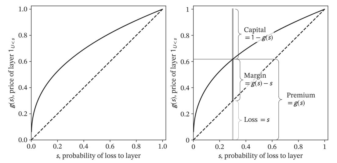
\(g(s)\) can be interpreted as the (ask) price to write a binary risk paying 1 with probability \(s\) and 0 otherwise
\(S(x) = \Pr(X>x)\), the survival function of a random variable \(X\) on sample space \(\Omega\)
- Loss cost \(\mathsf E[X] =\displaystyle\int_\Omega S(x)dx\)
\(g(S(x)) > S(x)\) is the risk-adjusted survival function
Spectral Pricing
Spectral pricing rule associated with a distortion \(g\) is given by \[\rho(X) = \int_\Omega g(S(x))dx\] It is intrepreted as a price, technical premium, risk-adjusted loss cost, or risk measure
Integration by parts trick gives an alternative expression
\[\rho(X) = \int_\Omega x g'(S(x))f(x)dx = \mathsf E[Xg'(S(X))]\]
which makes the spectral risk adjustment by \(g'(S(X))\) explicit
Distortion Functions and Insurance Statistics
Spectral Pricing Rules Have Nice Properties
Monotone: Uniformly higher risk implies higher price
Sub-additive: diversification decreases price
Comonotonic additive: no credit when no diversification; if out-comes imply same event order, then prices add
Law invariant: Price depends only on the distribution
All risk measures with these properties are SRM rules
SRM Pricing Adds Up Pricing by Layer
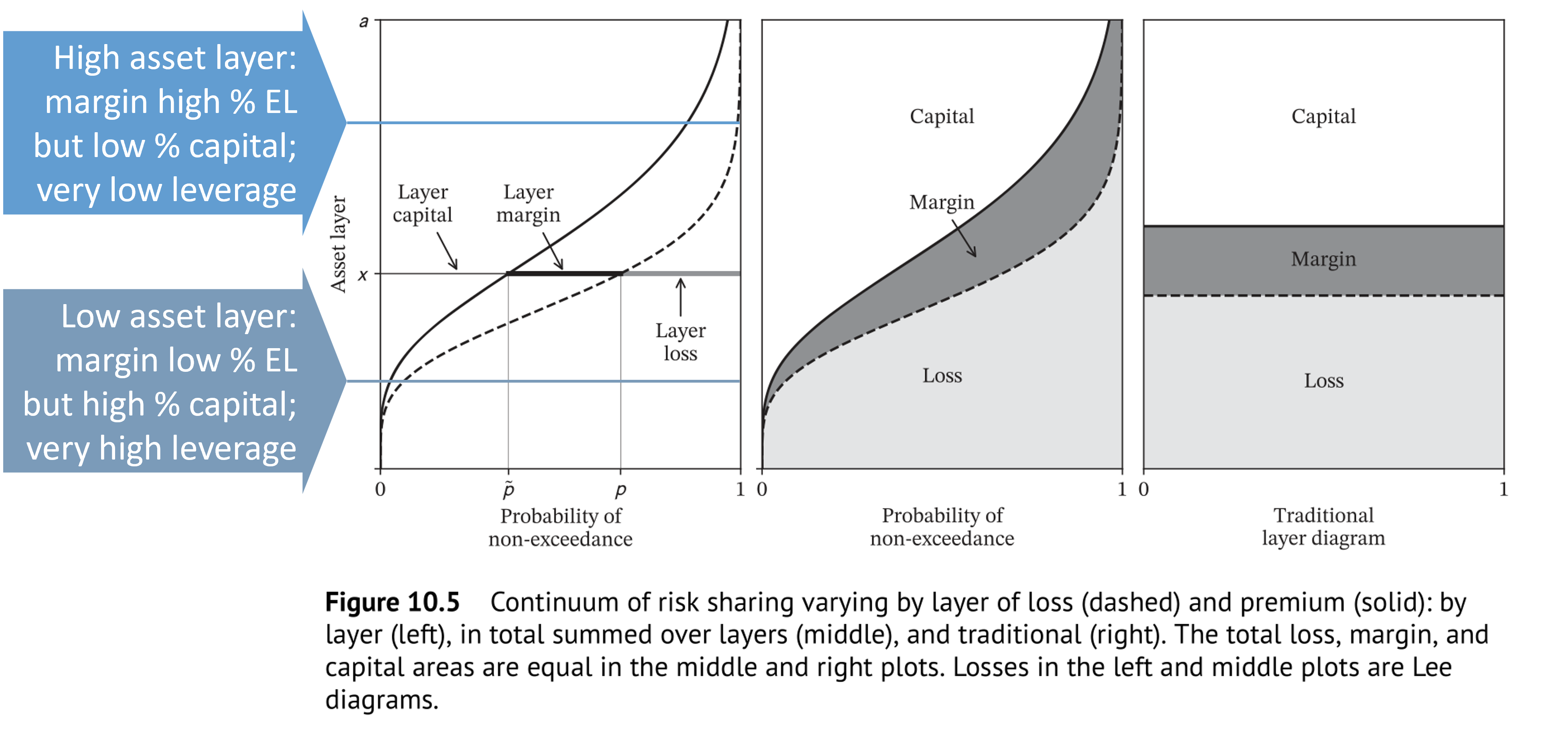
SRM Pricing has a Natural Allocation to Sub-units
- If \(X = \sum_i X_i\), define the natural allocation to unit \(i\) to be
\[\mathsf{NA}(X_i) = \mathsf E[X_i\, g'(S(X))]\]
Example: \(g(s)=\min(1, s / (1-p))\) corresponds to TVaR
- \(\rho(X) =\mathsf{TVaR}_p(X)\)
- \(\mathsf{NA}(X_i) = \mathsf{CoTVaR}_p(X_i)\)
The natural allocation pricing has nice properties
- It is natural because it involves no additional assumptions
- It adds-up because the sum of natural allocations is the original SRM price
- It equals marginal pricing when marginal pricing is well defined
CCoC Portfolio Pricing
CCoC = constant cost of capital, a common but thoughtless and problematic default
- Constant across layers of capital (debt, equity, etc.)
- Know not to be true…when computing WACC!
Various names: target return on capital or WACC or cost of capital set equal to \(r\)
General portfolio pricing rule: Premium = expected loss + cost of capital
CCoC Portfolio pricing rule: Premium = expected loss + \(r\times\) (amount of capital)
CCoC Portfolio Pricing with XTVaR Capital Standard
- CCoC implementation with XTVaR capital:
\[P(X) = \mathsf E[X] + r\, \mathsf{XTVaR}_p(X) = (1-r)\mathsf E[X] + r\, \mathsf{TVaR}_p(X)\]
Rule is a special case of SRM pricing
Corresponding distortion is \[g(s)=(1-r)s + r\min(1, s / (1-p))\]
- Weight \(1-r\) applied to all events: risk neutral part
- Weight \(r\) applied to \(p\)-tail events: extremely risk averse
- Example of a bi-TVaR, an average of two TVaRs, since \(\mathsf E[X] = \mathsf{TVaR}_0(X)\)
Easy to check \(\rho(X) = (1-r)\mathsf E[X] + r\mathsf{TVaR}_p(X)\)
XTVaR Natural Allocation
- Corresponding natural allocation is simply CoXTVaR pricing
\[\mathsf{NA}(X_i) = (1-r)\mathsf E[X_i] + r\, \mathsf{CoTVaR}(X_i) = \mathsf E[X_i] + r \, \mathsf{CoXTVaR}(X_i)\]
Shows SRM approach generalizes existing methods
Obvious question: What about using other distortions?
What does choice of distortion entail?
How can it be interpreted?
Distortions and Risk Appetite
Five “usual suspect” distortions
CCoC: \(g(s)=d + vs\) for \(s>0\) and \(g(0)=0\) where \(d=1/(1+r)\), \(v=1-d\) are discount rates
PH proportional hazard: \(g(s) = s^\alpha\), \(0 \le \alpha \le 1\)
Wang: \(g(s) = \Phi(\Phi^{-1}(s) +\lambda)\)
Dual: \(g(s) = 1 - (1 -s)^\beta\), \(\beta \ge 1\)
TVaR: \(g(s) = \min(1, s / (1-p))\)
Distortions and Risk Appetite
Calibrated distortion statistics for cat pricing example
| L | P | Q | COC | param | error | |
|---|---|---|---|---|---|---|
| method | ||||||
| ccoc | 46.6000 | 53.5652 | 46.4348 | 0.1500 | 0.1500 | 0.0000 |
| ph | 46.6000 | 53.5652 | 46.4348 | 0.1500 | 0.7205 | 0.0000 |
| wang | 46.6000 | 53.5652 | 46.4348 | 0.1500 | 0.3427 | 0.0000 |
| dual | 46.6000 | 53.5652 | 46.4348 | 0.1500 | 1.5952 | -0.0000 |
| tvar | 46.6000 | 53.5652 | 46.4348 | 0.1500 | 0.2713 | 0.0000 |
- Distortions easy to parameterize in Excel using Solver
Distortions and Risk Appetite
Calibrated distortion statistics for property risk example
| L | P | Q | COC | param | error | |
|---|---|---|---|---|---|---|
| method | ||||||
| ccoc | 1.0000 | 1.1765 | 0.8235 | 0.2143 | 0.2143 | 0.0000 |
| ph | 1.0000 | 1.1765 | 0.8235 | 0.2143 | 0.6203 | 0.0000 |
| wang | 1.0000 | 1.1765 | 0.8235 | 0.2143 | 0.4911 | 0.0000 |
| dual | 1.0000 | 1.1765 | 0.8235 | 0.2143 | 1.9677 | -0.0000 |
| tvar | 1.0000 | 1.1765 | 0.8235 | 0.2143 | 0.4334 | 0.0000 |
- For all distortions except PH, a higher parameter produces higher prices; for PH lower parameter produces higher prices
- These distortions are more expensive than the cat example
Algorithm for (Linear) Natural Allocation
- Compute unit average loss grouped by total loss & sum group probabilities
- Sort by ascending total loss (all values now distinct)
- Compute survival function S
- Apply distortion function g(S)
- Difference step 4 to compute risk adjusted probabilities Q
- Compute sum-products by unit and in total with respect to Q to obtain SRM pricing and natural allocation pricing by unit
Step 1 replaces \(X_i\) with the conditional expectation \(\mathsf E[X_i \mid X]\), a random variable defined by \(\mathsf E[X_i \mid X](\omega) = \mathsf E[X)i \mid X=X(ω)]\)
See PIR Algorithms 11.1.1 p.271 and 15.1.1, p.397 for more detail
See Why SRMs presentation for calculation details
Further Reading
Python source for presentation (RMarkdown) available on request
[1] for the theory of spectral risk measures, natural allocation, and implementation details
[2] for an introduction to the ideas behind the growth
[3] Modeling Standard of Practice for US Actuaries
References
1.
Mildenhall, S.J., Major, J.A.: Pricing insurance risk: Theory and practice. John Wiley & Sons, Inc. (2022)
2.
Peters, O.: Insurance as an ergodicity problem. Annals of Actuarial Science. 17, 215–218 (2023). https://doi.org/10.1017/S1748499523000131
3.
Actuarial Standards Board: Modeling. Actuarial Standard of Practice No. 56. (2019)