US vs European Economic Performance

1 Krugman’s US-Europe Tech Puzzle
TL;DR. A country specializing in fast-improving tradable goods can look especially strong in real GDP because it gets the production-volume credit. But as those goods become cheaper, much of the benefit is shared with importing countries through lower prices, so faster real GDP growth need not translate into equally faster current income or living standards.
This note explains a small trade model behind Paul Krugman’s “US-Europe paradox” post reproduced in Section 2. The model is useful, but very narrow. It shows how the US can look much stronger than Europe in real GDP growth if the US specializes in a sector with very rapid productivity growth, while Europe can still share much of the consumer benefit through trade. The model does not prove that Europe is doing well, that US outperformance is illusory, or that PPP comparisons settle the matter. The idea is illustrated with a global economy that moves from producing one car and one transistor per year to one car and one trillion transistors.
There are an important distinctions between three different types of GDP:
| Concept | Question |
|---|---|
| Current-price GDP | What is the current market value of domestic production? |
| Real GDP | How much has domestic production volume changed after removing price changes? |
| PPP income or PPP GDP | How much can income buy across countries with different price levels? |
The model’s main lesson is that real GDP is a production-volume measure, not a direct welfare measure. If the US produces the good whose quantity explodes, US real GDP gets the production credit. But if the good becomes much cheaper, foreign consumers also benefit. PPP is not relevant to the model.
1.1 Model Details
1.1.1 The Economy
There are two countries: the US and Europe. Each country has the same labor force. Labor is the only input into production. There is no capital, no land, no monopoly profit, no government, no taxes, no financial sector, and no international borrowing.
There are two goods:
| Good | Meaning In The Model | Concrete Example |
|---|---|---|
| \(N\) | Nontech good | cars |
| \(T\) | Tech good | transistors |
The symbols \(N\) and \(T\) denote physical quantities, not money values. If \(N=1\), the economy produces one car. If \(T=10^{12}\), the economy produces one trillion transistors.
The nontech good \(N\) is produced in both countries. The tech good \(T\) is produced only in the US. Both goods are tradable, meaning they can be bought in one country and sold in the other. Trade is costless, meaning there are no shipping costs, tariffs, regulatory frictions, exchange-rate spreads, delays, or distribution margins.
Costless trade implies a law of one price. If a car is cheaper in the US than Europe, buyers purchase cars in the US and ship them to Europe. That arbitrage continues until car prices are equal. The same logic applies to transistors.
1.1.2 The Numeraire
We can remove money from the model by measuring everything in cars. Set the price of one car equal to one: \[ p_N=1. \] Then all other prices are measured in cars. If \[ p_T=10^{-12}, \] one transistor costs \(10^{-12}\) cars, or one trillion transistors cost one car. This convention is called choosing a numeraire. A numeraire is the good used as the unit of account.
1.1.3 Production And Productivity
Let \(L_N\) be labor employed in car production, and let \(L_T\) be labor employed in transistor production. Labor is measured in worker-years. Let \(A_N\) be productivity in cars: \[ A_N=\frac{N}{L_N}. \] Its units are cars per worker-year. Finally, let \(A_T\) be productivity in transistors: \[ A_T=\frac{T}{L_T}. \] Its units are transistors per worker-year. The letter \(A\) is standard economist notation for a technology or productivity parameter. It does not have deep meaning; we could call the same quantities \(q_N\) and \(q_T\).
The production equations are: \[ N=A_N L_N, \] and \[ T=A_T L_T. \] Krugman’s key productivity assumptions are:
- Car productivity \(A_N\) is the same in the US and Europe;
- Car productivity does not grow;
- Transistor productivity \(A_T\) grows rapidly;
- Transistors are produced only in the US.
1.1.4 Wages And Prices
Let \(w\) be the wage, measured in cars per worker-year. A competitive firm pays a worker no more than the value of what the worker produces. If a worker produces \(A_N\) cars, and each car has price \(p_N\), then the worker’s output is worth \(p_NA_N\). With competition and no profits: \[ w=p_NA_N. \] Since \(p_N=1\), we get: \[ w=A_N. \] If one worker produces one car per year, then: \[ A_N=1, \] and the wage is one car per worker-year.
The same logic applies in tech: \[ w=p_TA_T. \] Therefore the transistor price satisfies: \[ p_T=\frac{w}{A_T}. \] Since \(w=A_N\), we have: \[ p_T=\frac{A_N}{A_T}. \] This equation is the center of the model. If car productivity stays fixed and transistor productivity explodes, the price of transistors collapses.
1.1.5 Why The Same Wage Appears In Both Countries
Krugman’s wage-equalization sentence is easy to mistrust unless we spell out every step. The nontech good \(N\) is tradable, so it has the same price in the US and Europe: \[ p_N^{US}=p_N^{EU}. \] Nontech productivity is the same: \[ A_N^{US}=A_N^{EU}. \] Competitive wages in the nontech sector are therefore: \[ w_N^{US}=p_NA_N, \] and \[ w_N^{EU}=p_NA_N. \] Hence: \[ w_N^{US}=w_N^{EU}. \] Inside the US, labor can move between the car sector and the tech sector. If tech pays more than cars, workers leave cars for tech. If cars pay more than tech, workers leave tech for cars. With homogeneous labor and free movement across sectors: \[ w_T^{US}=w_N^{US}. \] So the common nontech sector pins the wage, and tech prices adjust to make the tech sector able to pay that wage. This is not a claim that real-world US and EU wages must be equal. It is a model implication produced by equal nontech productivity, costless trade, homogeneous labor, and perfect competition.
1.1.6 Demand
Consumers in both countries consume both cars and transistors. Krugman uses Cobb-Douglas preferences. The important implication is that consumers spend a fixed share of income on each good. Let \(\alpha\) be the fraction of income spent on tech. Then:
| Expenditure | Value |
|---|---|
| Spending on \(T\) | \(\alpha Y\) |
| Spending on \(N\) | \((1-\alpha)Y\) |
The share \(\alpha\) is dimensionless. It is a fraction, such as \(1/4\) or \(1/2\). A fixed expenditure share does not mean a fixed number of transistors. If transistors get cheaper, the number of transistors purchased rises. If income is one car and \(\alpha=1/2\), spending on tech is half a car. If one transistor costs one car, the consumer buys half a transistor. If one transistor costs \(10^{-12}\) cars, the consumer buys half a trillion transistors. Thus the model does allow demand for tech to rise as tech gets cheaper. What stays fixed is the share of income spent on tech, not the physical quantity of tech consumed.
1.1.7 Employment
Each country has labor force \(L\). Europe produces only cars, so: \[ L_N^{EU}=L. \] The US produces both cars and transistors, so: \[ L_N^{US}+L_T^{US}=L. \] World income is \(2wL\), because the two countries have the same labor force and the same wage. World spending on tech is: \[ 2\alpha wL. \] Each US tech worker produces value \(w\), because \(p_TA_T=w\). Hence the amount of US labor needed in tech is: \[ L_T^{US}=2\alpha L. \] (The US tech labor share is determined by world demand for tech. World income is \(2wL\), consumers spend share \(\alpha\) on tech, so world tech spending is \(2\alpha wL\); each US tech worker produces value \(p_TA_T=w\), hence \(wL_T^{US}=2\alpha wL\) and \(L_T^{US}=2\alpha L\).)
This requires \(\alpha<1/2\) if the US is also to produce some cars. That is why the assumption \(\alpha<1/2\) matters. It keeps the US in both sectors, so the common car sector visibly pins the wage.
If we use \(\alpha=1/2\) for a clean numerical example, the US puts all labor into tech. The wage-pinning logic then works as a limiting case, or as an outside option: US workers could produce cars at the same productivity if needed. To avoid that corner case exactly, replace \(1/2\) by \(0.49\) everywhere. The intuition is unchanged.
1.1.8 Current-Price GDP
Current-price GDP is the value of domestic production at current prices. With two goods: \[ Y=p_NN+p_TT. \] In Europe, only cars are produced: \[ Y_{EU}=p_NA_NL. \] Since \(p_NA_N=w\), this is: \[ Y_{EU}=wL. \] In the US: \[ Y_{US}=p_NA_NL_N^{US}+p_TA_TL_T^{US}. \] Since \(p_NA_N=w\) and \(p_TA_T=w\), this becomes: \[ Y_{US}=wL_N^{US}+wL_T^{US}=wL. \] Therefore: \[ Y_{US}=Y_{EU}. \] The US may produce a spectacular amount of tech, but if tech prices fall in inverse proportion to tech productivity, the current market value of US output need not rise relative to Europe.
1.1.9 Real GDP
Real GDP tries to measure output volume, not current market value. It asks: how much more production is there after removing price changes? This is a useful question, but it is not the same as asking how rich people are, how much income they command at current prices, or how much welfare they get from consumption.
In the model, the US produces the good whose physical quantity explodes. So US real GDP grows quickly. Europe imports the cheap tech, so Europe benefits as a consumer, but Europe does not receive the same production-side real GDP credit.
The result is not necessarily an error in real GDP. It is a reminder that real GDP is an output-volume index. When relative prices change dramatically, output-volume indexes and current-value measures tell very different stories.
1.1.10 PPP
PPP means purchasing power parity. PPP comparisons adjust incomes across countries for differences in price levels.
In the pure two-good model, both goods are costlessly tradable, and both countries face the same prices. In that special world, PPP does almost nothing. Same wage, same prices, same purchasing power.
PPP matters in the real world because many goods are not costlessly tradable: housing, medical services, legal services, education, haircuts, restaurants, local transport, government services, and many personal services. If these prices differ between countries, equal nominal income does not imply equal purchasing power.
Thus PPP is not a fix for real GDP. It answers a different question. Real GDP asks about domestic production volume over time. PPP asks what income can buy across countries.
1.2 Example: One Car And One Trillion Transistors
1.2.1 Year 1
Take one car as the unit of account: \[ p_N=1. \] Suppose one worker can make one car per year: \[ A_N=1. \] Suppose one worker can make one transistor per year: \[ A_T=1. \] The wage is: \[ w=p_NA_N=1. \] So the wage is one car per worker-year.
The transistor price is: \[ p_T=\frac{w}{A_T}=1. \] So one transistor costs one car.
For the cleanest illustration, suppose each country has one worker and each consumer spends half of income on cars and half on transistors. This uses the limiting case \(\alpha=1/2\). The exact Krugman assumption \(\alpha<1/2\) gives the same conclusion with slightly messier numbers.
Each country has income equal to one car. Each country consumes:
| Good | Spending | Price | Quantity |
|---|---|---|---|
| Cars | 0.5 cars | 1 car per car | 0.5 cars |
| Transistors | 0.5 cars | 1 car per transistor | 0.5 transistors |
World consumption is one car and one transistor. The US produces the transistor. Europe produces the car. Trade balances: the US exports half a transistor and imports half a car; Europe exports half a car and imports half a transistor.
Current-price GDP is:
| Country | Output | Current Price | Current-Price GDP |
|---|---|---|---|
| US | 1 transistor | 1 car per transistor | 1 car |
| Europe | 1 car | 1 car per car | 1 car |
Both countries have current-price GDP equal to one car.
1.2.2 Year 2
Now transistor productivity explodes: \[ A_T=10^{12}. \] One US worker now produces one trillion transistors per year. Car productivity remains: \[ A_N=1. \] The wage remains pinned by car production: \[ w=1. \] The transistor price becomes: \[ p_T=\frac{1}{10^{12}}. \] One transistor costs one trillionth of a car. One trillion transistors cost one car.
Each country still has income equal to one car. Each country spends half its income on cars and half on transistors:
| Good | Spending | Price | Quantity |
|---|---|---|---|
| Cars | 0.5 cars | 1 car per car | 0.5 cars |
| Transistors | 0.5 cars | \(10^{-12}\) cars per transistor | \(0.5 \times 10^{12}\) transistors |
Both countries are better off in a real consumption sense. Each still consumes half a car, but each now consumes half a trillion transistors instead of half a transistor.
Current-price GDP is still:
| Country | Output | Current Price | Current-Price GDP |
|---|---|---|---|
| US | \(10^{12}\) transistors | \(10^{-12}\) cars per transistor | 1 car |
| Europe | 1 car | 1 car per car | 1 car |
So the US does not become richer than Europe in current-price GDP. The value of US output remains one car because the quantity of transistors rises by a factor of \(10^{12}\) while the price per transistor falls by the same factor.
1.2.3 Why The US Looks Richer In Real GDP
If we focus on production volume, the US economy has changed dramatically. It used to produce one transistor. It now produces one trillion transistors. On a real output measure, that is enormous growth.
If we foolishly valued today’s transistor output at the old price of one car per transistor, US output would appear to be worth: \[ 10^{12} \text{ cars}. \] That fixed-old-price calculation is obviously absurd as a welfare measure. No sane buyer values today’s ordinary transistor at its early historical price. Modern chained indexes are designed to avoid using ancient prices forever.
But even a better real-output index faces the same conceptual issue: it records a huge increase in the volume of tech output. That is a production fact. The separate economic question is who benefits from the cheaper tech. In this example, both countries benefit, because both consume the cheaper transistors.
Thus the apparent contradiction is:
| Perspective | US Compared With Europe |
|---|---|
| Tech production volume | US is vastly ahead |
| Current-price GDP | US and Europe remain equal |
| Consumption possibilities | Both countries improve |
| PPP in the toy model | Same as current purchasing power, because prices are common |
| Welfare | Higher in both countries, but not uniquely higher in the US |
1.3 What The Model Says
The model says that the following facts can coexist:
- the US specializes in tech;
- tech productivity grows very rapidly;
- US real GDP grows faster than European real GDP;
- tech prices fall rapidly;
- Europe imports cheaper tech;
- current-price GDP does not diverge;
- PPP living standards need not diverge.
The mechanism is simple. Productivity growth in tech raises the quantity of tech output and lowers the relative price of tech. The country producing tech gets the real production-growth credit. But consumers in both countries buy the cheaper tech.
The model is therefore a warning against the claim:
US real GDP grew faster than European real GDP, therefore US living standards must have pulled decisively ahead of Europe’s.
Krugman’s answer is: not necessarily. If faster US real GDP growth reflects production of a fast-improving tradable good, then some of the gain is exported through lower prices.
1.4 What The Model Does Not Say
The model does not say Europe is economically healthy.
It does not say US out-performance is fake.
It does not say PPP measures are perfect.
It does not say real GDP is useless.
It does not say tech dominance is unimportant.
It does not say US tech workers are not highly paid.
It does not say monopoly profits, intellectual property rents, capital ownership, and stock-market gains are irrelevant in the real world.
It says only that production-side real GDP growth can overstate the domestic living-standard advantage of specializing in a rapidly improving tradable sector.
That is a narrow but useful claim.
1.5 Critique
1.5.1 The Model Is Engineered To Equalize Current Income
The equal-income result does not fall from the sky. It is built into the assumptions. The current-price GDP equality follows from: \[ Y_{US}=wL, \] and \[ Y_{EU}=wL. \] The same wage comes from equal nontech productivity and costless trade. The same GDP comes from equal labor forces and labor-only production. There are no profits, no capital income, no rents, and no ownership claims. This is not a realistic description of the US tech economy. It is a deliberately stripped-down benchmark.
1.5.2 Tech Wages Are High In The Real World
Real-world tech wages are high because the assumptions of the toy model fail. Tech workers are not homogeneous with all other workers. Skills are scarce. Firms have market power. Intellectual property creates rents. Equity compensation gives workers claims on future profits. Agglomeration raises productivity and pay in tech clusters. Housing costs and local labor markets matter. Immigration limits prevent full wage equalization. The model’s wage result is not an empirical claim that tech and nontech workers receive the same wage. It is a competitive benchmark.
1.5.3 Tech Is Often An Intermediate Input
The model treats cars and transistors as separate final goods. Reality is messier. Cars contain chips. Banks use software. Hospitals use cloud computing. Logistics uses sensors. Shops use payment networks. Almost every sector uses information technology.
If tech is an intermediate input into nontech production, then cheaper tech can raise productivity in the nontech sector too. Europe may then get measured production gains in nontech even if it does not produce the underlying chips or software. This complicates the simple US-produces-tech, Europe-consumes-tech story.
1.5.4 PPP Is Not A Magic Truth Machine
PPP comparisons are valuable, but they are not mechanical facts. They depend on price baskets, quality adjustments, housing costs, health care, government services, taxes, and nontraded goods. PPP is especially hard when goods differ in quality or when public services are provided differently. In the pure model, PPP is trivial because all goods are tradable and all prices are the same. In the real world, PPP matters precisely because the pure model is false. Thus PPP should not be treated as the final answer. It is one useful lens.
1.5.5 Real GDP: Treat with Care
Real GDP is not simply nonsense. It answers a coherent question: how much has domestic production volume changed after adjusting for prices? The problem is that people often hear “real GDP” as “real prosperity.” Those are not the same. Real GDP is especially tricky when a sector undergoes dramatic quality change and price collapse.
For tech, the measurement problem is severe. A “computer,” “chip,” “phone,” or “software service” changes quality over time. Statistical agencies use quality adjustments to estimate constant-quality prices. Such adjustments are necessary, but they are also judgmental.
Krugman’s model exploits a real distinction: output volume can rise much faster than current value. The rhetorical risk is that the model makes a narrow measurement point sound like a broad verdict on US versus European economic performance.
1.5.6 The Trade Balance Is Simple Only Because The Model Is Simple
In the numerical example, trade balances naturally. The US exports tech worth half a car and imports cars worth half a car. Europe does the reverse. In reality, countries can run trade deficits or surpluses. They can borrow, lend, hold reserve currencies, receive investment income, or pay for imports with asset claims. Exchange rates move. Multinational firms book profits in low-tax jurisdictions. Supply chains cross borders many times. None of that appears in the toy model.
1.5.7 Narrow Conclusions
The model proves that one inference is unsafe: faster US real GDP growth does not automatically imply an equal increase in US living standards relative to Europe. But the model does not prove the opposite. It does not prove that Europe is keeping up in a broad welfare sense.
Krugman’s model is a useful warning about interpreting real GDP growth in a world of fast-improving tradable technology. It is not a general vindication of European economic performance, and it is not a complete account of US tech dominance.
1.6 Summary
The whole model reduces to three equations: \[ w=p_NA_N, \] \[ w=p_TA_T, \] and therefore \[ \frac{p_T}{p_N}=\frac{A_N}{A_T}. \] If car productivity \(A_N\) stays fixed and transistor productivity \(A_T\) rises enormously, the relative price of transistors falls enormously.
The US produces the transistors, so US real GDP records enormous production growth. Europe imports the cheaper transistors, so Europe shares the consumer gain. Current-price GDP need not diverge, because the larger transistor quantity is offset by the lower transistor price. The producer gets the real-output credit, but consumers everywhere get the cheaper good. That is an important point and it is also much narrower than saying Europe is doing fine.
1.8 Variable Table
| Symbol | Definition | Units In The Example |
|---|---|---|
| \(N\) | Quantity of nontech output | cars per year |
| \(T\) | Quantity of tech output | transistors per year |
| \(L\) | Total labor force in a country | worker-years per year |
| \(L_N\) | Labor employed in nontech production | worker-years per year |
| \(L_T\) | Labor employed in tech production | worker-years per year |
| \(A_N\) | Nontech labor productivity | cars per worker-year |
| \(A_T\) | Tech labor productivity | transistors per worker-year |
| \(p_N\) | Price of the nontech good | cars per car, normalized to 1 |
| \(p_T\) | Price of the tech good | cars per transistor |
| \(w\) | Wage | cars per worker-year |
| \(Y\) | Current-price GDP | cars per year |
| \(\alpha\) | Share of income spent on tech | dimensionless fraction |
| \(Y_{US}\) | US current-price GDP | cars per year |
| \(Y_{EU}\) | European current-price GDP | cars per year |
1.9 Definitions Of Terms Of Art
| Term | Meaning |
|---|---|
| Numeraire | The good used as the unit of account; here, one car |
| Current-price GDP | Domestic output valued at current market prices |
| Real GDP | An index of domestic output volume after removing price changes |
| PPP | Purchasing power parity, an adjustment for cross-country price-level differences |
| Tradable good | A good that can be bought in one country and sold in another |
| Costless trade | Trade with no shipping costs, tariffs, frictions, delays, or margins |
| Law of one price | Costless arbitrage equalizes prices across locations |
| Productivity | Output per unit of input, here output per worker-year |
| Cobb-Douglas preferences | Preferences that imply fixed expenditure shares |
| Expenditure share | The fraction of income spent on a good |
| Real output | Output measured as quantity or volume rather than current value |
| Current value | Quantity multiplied by the current price |
| Welfare | Economic well-being, which depends on consumption possibilities, distribution, leisure, public goods, and many other factors beyond GDP |
2 Original Post
I recently wrote about the European economy, and how the widespread narrative that says that Europe is in decline isn’t supported by the evidence. As I noted, conventional measures of growth in GDP per capita have favored the United States since 2000:
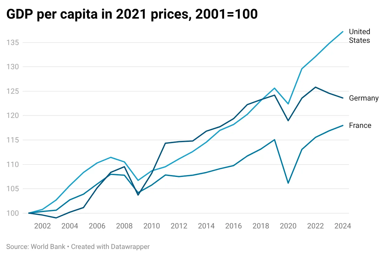
But European relative GDP per capita measured at PPP has not declined:
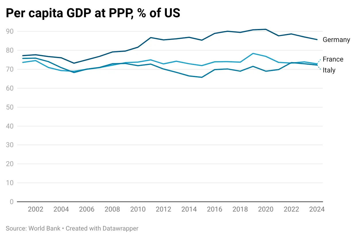
Call this the US-Europe paradox.
Of course, it isn’t really a paradox. It makes perfect sense given US dominance of sectors that are experiencing rapid productivity growth, which leads to a rise in relative US GDP at constant prices but doesn’t translate into a rise in relative GDP at current prices. But I worry somewhat that my attempt to explain what’s going on in terms that non-economists might be able to follow may, um, paradoxically have made it less clear to economists. So this note lays the story out economics-professor style, with a bit of math.
Economese from here on.
A stylized model of the US-Europe paradox
Imagine a world consisting of two countries, US and EU. Assume for the sake of simplicity that labor is the only factor of production, and that the two countries have equal labor forces.
There are two goods, tech (T) and nontech (N). Both are costlessly tradable. Preferences are Cobb-Douglas, with consumers in both countries spending a constant share 𝜏<1/2 of their income on T.
Labor productivity in the production of N is assumed to be the same in both countries, and again for simplicity I assume zero productivity growth in that sector. Because productivity is the same and N is tradable, this ensures that wages are the same in the two countries, and hence that GDP in current prices is the same.
However, there is technological progress in tech, T.
I assume that US has a comparative advantage in T, and hence that all T is produced there. It doesn’t matter for this model what the source of that comparative advantage is, although in the real world it has a lot to do with the positive externalities generated by industrial clusters.
Crucially for this analysis, T experiences more rapid technological progress than N. I assume that productivity in that sector rises at a rate ⍴, versus zero in N.
Given these assumptions, what does the model imply for measured growth and relative performance?
As I’ve set it up, the model implies that all T will be concentrated in US. Because T attracts a share 𝜏 of world spending, it will also account for a share 𝜏 of world GDP, and hence 2𝜏 of US GDP.
Given this, technological progress in T implies rising US real GDP, measured the way we actually calculate it — as growth in “chained” constant prices — at a rate of 2𝜏𝜌. Growth in EU real GDP is zero. (We could obviously add in some growth in N productivity to make this number positive.) Yet relative GDP at current prices remains 1.
Oh, and real wages rise at the rate 𝜏𝜌 in both nations.
And that’s the US-Europe paradox. US dominance in tech leads to higher measured growth in the United States than in Europe, but not to a divergence in relative GDP or living standards.