| s | gs | a | b | eta- | eta+ |
|---|---|---|---|---|---|
| 0.02704242 | 0.6642399 | 24.56289 | - | 1 | 0.04510946 |
| 0.202685 | 0.858855 | 1.108018 | 0.6342764 | 0.2614861 | 0.06931349 |
| 0.683247 | 1 | 0.2937082 | 0.7993248 | 0.2006752 | - |
| 1 | 1 | - | 1 | - | - |
On Submultiplicative Distortions
notes
mathematics
risk
llm
Submultiplicativity, diagonal tests, and exact maxima for piecewise-linear distortions.
Motivation
Pre-LLM, I worked on this problem on-and-off for several weeks. Post-LLM, I solved it in two days. Or, should that be, “We solved it”? Here’s the story.
Distortion functions \(g\) like the Wang or proportional hazard sit at the center of the theory of coherent, convex, and spectral risk measures. They are simple objects, but when one starts asking structural questions about whether inequalities such as \[ g(st)\ \stackrel{?}{\le}\ g(s)\,g(t), \] hold, some tricky geometry appears. This particular question, asking whether \(g\) is submultiplicative, has interesting implications for how \(g\) prices multi-period risk, making it important to be able to determine whether or not \(g\) is submultiplicative.
This post documents my investigation of a conjecture about submultiplicativity that initially looks true (and survives a lot of numerical experimentation), but is ultimately false. It shows the reductions and algorithms that make it possible to search reliably and successfully for counterexamples.
The analysis hinges on an understanding the function \[ h(s,t)=g(st)-g(s)g(t), \] its behavior on a partition of \([0,1]^2\) into “knot regions”, and how to compute \(\max h\) exactly (for piecewise-linear \(g\)) without brute force gridding.
Distortions and piecewise-linear distortions
A distortion is a function \(g:[0,1]\to[0,1]\) that is
- nondecreasing,
- concave, and
- normalized: \(g(0)=0\) and \(g(1)=1\).
The Wang and proportional hazard distortions are two well-known examples. Distortions induce coherent and convex risk measures via Choquet integration and, through Kusuoka-type representations, connect to spectral risk measures. In particular, TVaR appears as the “atomic” building block.
TVaR distortions
For \(0\le p<1\), the TVaR distortion at level \(p\) is the piecewise-linear function \[ t_p(s) = 1\wedge \frac{s}{1-p} = \min\!\left(1,\frac{s}{1-p}\right), \qquad s\in[0,1]. \] It is linear on \([0,1-p]\) with slope \(1/(1-p)\) and constant \(1\) on \([1-p,1]\).
There is a limiting case at \(p=1\) producing the step function \(t_1(s)=1_{\set{s>0}}\), corresponding to max, but in much of what follows I exclude this case because it introduces a jump at \(0\) and it is easy to see that discontinuous distortions are not submultiplicative.
Piecewise-linear distortions as finite mixtures of TVaR distortions
A piecewise-linear distortion is a finite convex combination of TVaR distortions: \[ g(s)=\sum_{k=1}^n w_k\,t_{p_k}(s), \] where the probability levels \(0\le p_k<1\), and the weights are positive and sum to 1 \[ w_k\ge 0, \qquad \sum_{k=1}^n w_k=1. \] Such \(g\) is continuous, concave, and piecewise affine. All distortions are convex (integral) combinations of TVaR; these are just the finite combinations. (The reason is fascinating and fundamental: TVaRs are extreme points in the convex set of distortions, and any point in a convex set is a weighted average of extreme points.)
Equivalently, \(g\) is determined by a finite set of knot points \[ x_k=1-p_k \in (0,1), \] together with the values \(g(x_k)\). Between adjacent knots, \(g\) is affine (a straight line).
When implementing, it is convenient to represent \(g\) by its knot table \[ (x_0,g(x_0)), (x_1,g(x_1)),\dots,(x_n,g(x_n)), \] with \(x_0=0\), \(x_n=1\), and linear interpolation in between.
On each interval \([x_r,x_{r+1}]\), \[ g(u)=a_r u + b_r, \] where \(a_r\) is the slope on that segment and \(b_r\) the intercept.
Concavity imposes that the slopes decrease \[ a_0 \ge a_1 \ge \cdots \ge a_{n-1}\ge 0, \] and the intercepts increase from zero to \(1\).
At a knot \(x\), the left and right segment coefficients satisfy a continuity identity. Writing left coefficients \((a^-,b^-)\) and right coefficients \((a^+,b^+)\), concavity gives \(a^->a^+\) and continuity gives \[ b^+ - b^- = (a^- - a^+)\,x. \] This simple relation becomes surprisingly useful when analyzing derivatives across knot boundaries.
Submultiplicativity and diagonal submultiplicativity
Define \[ h(s,t)=g(st)-g(s)g(t), \qquad (s,t)\in[0,1]^2. \]
Submultiplicativity (SBM)
A distortion \(g\) is submultiplicative (SBM) if \[ g(st)\le g(s)\,g(t)\qquad \text{for all } s,t\in[0,1], \] equivalently \[ h(s,t)\le 0\qquad \text{for all }(s,t)\in[0,1]^2. \]
Diagonal submultiplicativity (DSBM)
A distortion \(g\) is diagonally submultiplicative (DSBM) if \[ g(s^2)\le g(s)^2\qquad \text{for all } s\in[0,1], \] equivalently \[ h(s,s)\le 0 \qquad \text{for all } s\in[0,1]. \]
It is immediate that SBM implies DSBM by restricting to the diagonal \(t=s\).
The conjecture
The conjecture that starts this whole story:
Conjecture 1 For a continuous piecewise-linear distortion \(g\), \[ \text{$g$ is SBM} \quad\Longleftrightarrow\quad \text{$g$ is DSBM.} \]
The direction SBM \(\Rightarrow\) DSBM is trivial. The content is the reverse implication DSBM \(\Rightarrow\) SBM.
Intuitively, the conjecture is tempting because:
- TVaR distortions \(t_p\) with \(0<p<1\) are SBM.
- Many mixtures preserve “diagonal dominance” empirically.
- In smaller families (e.g. biTVaR), violations always manifest on the diagonal.
A cautionary tale: naïve numerical search and fake counterexamples
My first numerical experiments used random samples in \((s,t)\) to test whether \(h(s,t)\) becomes positive.
This approach can fail badly.
The reason is geometric: for piecewise-linear \(g\), the sign changes of \(h\) can occur in very narrow regions, often hugging boundaries between knot regions. A random scatter in \([0,1]^2\) can miss these thin positive sets entirely, leading to a false conclusion that \(\max h \le 0\).
In other words: a distortion may be non-SBM, but the “area” where \(h>0\) is so small that naïve Monte Carlo misses it.
This motivates an exact computation of \(\max h\) for piecewise-linear distortions.
Partition of \([0,1]^2\) into knot regions
Let the knot set for \(g\) be \(0=x_0 < x_1 < \cdots < x_n=1\).
The unit square \([0,1]^2\) is partitioned by:
- vertical lines \(s=x_i\) where the affine form of \(g(s)\) changes,
- horizontal lines \(t=x_j\) where the affine form of \(g(t)\) changes, and
- hyperbolas \(st=x_k\) where the affine form of \(g(st)\) changes.
A knot region is a subset where the segment indices of \(s\), \(t\), and \(st\) are fixed: \[ s\in[x_i,x_{i+1}],\quad t\in[x_j,x_{j+1}],\quad st\in[x_k,x_{k+1}]. \]
On such a region, write \[ g(s)=a_i s + b_i,\qquad g(t)=a_j t + b_j,\qquad g(st)=a_k st + b_k. \]
Then on that region, \[ \begin{aligned} h(s,t) &= (a_k st+b_k)-(a_i s+b_i)(a_j t+b_j) \\ &= (a_k-a_i a_j)\,st - a_i b_j\,s - a_j b_i\,t + (b_k-b_i b_j). \end{aligned} \] So \(h\) is bilinear on each region: \[ h(s,t) = \alpha\,st + \beta\,s + \gamma\,t + \delta. \]
This has a decisive consequence:
- a bilinear function on a rectangle has no strict interior extremum (unless degenerate), and
- therefore extrema on a region occur on the region boundary.
So the search for \(\max h\) reduces to evaluating \(h\) on the boundaries of all regions.
Boundary reduction and the role of hyperbolas
Cell boundaries consist of:
- vertical or horizontal segments where \(s=x_i\) or \(t=x_j\),
- arcs along hyperbolas \(st=x_k\).
Vertical/horizontal segments reduce to evaluating an affine function on an interval, so extrema occur at endpoints (knot intersections). This leads to a finite set of candidate points: the knot grid \((x_i,x_j)\).
The genuinely new feature comes from hyperbola boundaries.
Restriction of \(h\) to a hyperbola boundary
Fix \(c\in(0,1)\) and consider the hyperbola \(st=c\).
Along this curve, define \[ f(s)=h(s,c/s)=g(c)-g(s)g(c/s),\qquad s\in[c,1]. \]
On an interval where \(g(s)\) and \(g(c/s)\) are both affine, \[ g(s)=a_i s+b_i,\qquad g(c/s)=a_j \frac{c}{s} + b_j, \] we have \[ \begin{aligned} f(s) &= g(c)-(a_i s+b_i)\Bigl(a_j \frac{c}{s}+b_j\Bigr) \\ &= \text{const} - (a_i b_j)\,s - (b_i a_j)\,\frac{c}{s}. \end{aligned} \] So on each such arc, \[ f(s)=\text{const} - A s - \frac{B}{s}, \qquad A=a_i b_j,\quad B=b_i a_j c, \] and hence \[ f''(s)=-\frac{2B}{s^3}\le 0. \] Therefore \(f\) is concave on each arc.
Consequently, on each arc:
- \(f\) attains its maximum at an endpoint or at the unique stationary point (if it lies in the arc interior).
The stationary point solves \[ f'(s)=0 \quad\Longleftrightarrow\quad -A + \frac{B}{s^2}=0 \quad\Longleftrightarrow\quad s^2=\frac{B}{A}=\frac{a_j b_i c}{a_i b_j}. \]
Thus, in addition to endpoints, one must include the candidate point \[ s_*=\sqrt{\frac{a_j b_i c}{a_i b_j}},\qquad t_*=\frac{c}{s_*}, \] provided \(s_*\) lies in the \(s\)-segment \([x_i,x_{i+1}]\) and \(t_*\) lies in the \(t\)-segment \([x_j,x_{j+1}]\).
This is the exact place where interior maximizers enter the overall algorithm: they are interior points of hyperbola arcs, not interior points of 2D regions.
Counting candidates and the speedup
Suppose \(g\) has \(n\) segments (equivalently \(n+1\) knots including endpoints). A naïve grid search of size \(N\times N\) is \(O(N^2)\) evaluations and does not provide any guarantee.
The exact boundary approach produces a candidate set whose size is quadratic in \(n\):
- knot grid points: \(n^2\),
- hyperbola–knot-line intersections: for each knot \(c\), intersect with each knot line \(s=x_i\) and \(t=x_j\), giving \(O(n^2)\),
- stationary points: for each knot \(c\) and each segment pair \((i,j)\), potentially one point, giving \(O(n^3)\) in the worst case, with many pruned by feasibility checks.
Even at \(n=128\) (a common regime in my experiments), this is tractable, and it is exact: no thin positive region is missed. To search numerically requires \(N\gg n\) and is not determinative.
This algorithmic reframing is the main practical insight: understanding the geometry of \(h\) makes the search fast and reliable.
The elasticity function \(\eta\) and internal turning points
An associated diagnostic that turns out to be helpful is the elasticity function. For a general \(y=g(x)\), the elasticity of \(y\) with respect to \(x\) is the dimensionless quantity \[ \frac{d\log y}{d\log x} = \frac{d\log g(x)/dx}{d\log x/dx} = \frac{g'(x)/g(x)}{1/x} = \frac{xg'(x)}{g(x)}. \] Elasticity is used in economics to measure price sensitivity. Elasticity \(\alpha\) means a 1% change in \(x\) produces an \(\alpha\)% change in \(g(x)\).
On a segment where \(g(u)=b+m u\), the elasticity function equals \[ \eta(u):=\frac{u g'(u)}{g(u)}=\frac{m u}{b+m u}. \] Within a fixed affine segment, \(\eta\) is strictly increasing in \(u\), and at a knot, the slope \(m\) drops, so \(\eta\) jumps downward. Thus, \(\eta\) has a “sawtooth” shape: rising within segments, jumping down at knots.
Why does \(\eta\) appear naturally? Because on a hyperbola \(st=c\), stationary points of \(f(s)=g(c)-g(s)g(c/s)\) satisfy \[ f'(s)=0 \quad\Longleftrightarrow\quad \eta(s)=\eta(t), \qquad t=c/s, \] at least when both \(s\) and \(t\) lie in fixed affine pieces.
This makes \(\eta\) a useful interpretive tool:
- internal turning points on hyperbola arcs correspond to matches \(\eta(s)=\eta(t)\),
- because \(\eta\) jumps down at knots, such matches can occur with \(s\ne t\) when \(s\) and \(t\) lie in different regions.
A further trick that makes the symmetry transparent.
Hyperbola parameterization by \(x\)
Fix \(c\) and set \(u=\sqrt c\). Parameterize \(st=c\) by \[ s=u e^x,\qquad t=u e^{-x}. \] Then \(x=0\) is the diagonal \(s=t=u\), and the map \(x\mapsto -x\) swaps \(s\) and \(t\). This makes plots of \(h\) along hyperbolas against \(x\) look symmetric by construction, and it becomes easier to see multiple local maxima and their relation to knot crossings. We use this in the illustrations below.
A structural observation: why at least three knots matter
The sawtooth shape of \(\eta\) clarifies why certain small families cannot produce counterexamples:
- with too few knot regions, there are not enough downward jumps to create multiple solutions of \(\eta(s)=\eta(t)\) off-diagonal,
- in particular, for some small classes (e.g. biTVaR) the “bad behavior” is tightly constrained and violations tend to (must for biTVaR) appear on the diagonal.
But with many knot points (large \(n\)), the hyperbola traverses many knot regions. The function \(h\) along a single hyperbola becomes piecewise concave with many stitched caps, and it is entirely possible for \(\max_{st=c} h(s,t)\) to be positive while the diagonal value \(h(\sqrt c,\sqrt c)\) remains negative. This phenomenon invalidates the conjecture.
The outcome: the conjecture is false
After replacing naïve random probing with the exact maxima computation described above, counterexamples become easy to find:
- distortions \(g\) for which \(\max_{s,t} h(s,t) > 0\) (so \(g\) is not SBM),
- while the diagonal excess \(d(s)=g(s^2)-g(s)^2\) is never positive (so \(g\) is DSBM).
In such examples, \(d(s)\) is typically negative away from the endpoints and equals \(0\) only at \(s=0\) and \(s=1\).
Examples
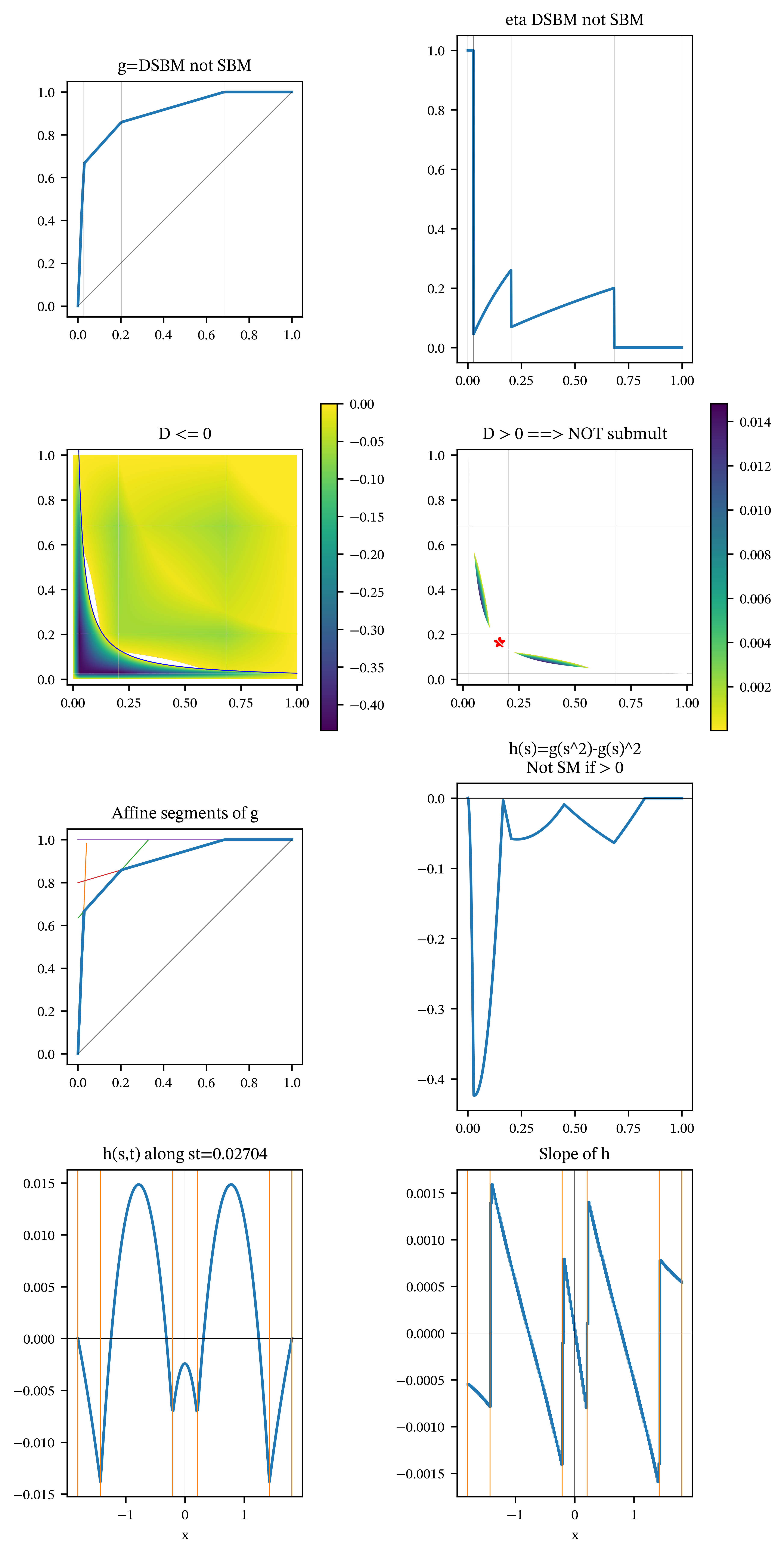
The diagonal conjecture is true for biTVaRs, so any counterexample needs at least three knot points. Counter-examples are easy to find, and one is defined by the \(p\) \[ p = (0.31675297, 0.79731504, 0.97295758) \] and \(w\) values \[ w = (0.20067524, 0.16504839, 0.63427637). \] The knots are at the points \(1-p\). Table 1 shows the corresponding slopes and constants defining the affine segments. The facets of Figure 1 illustrate the following, indexed by \((r,c)\) for the plot in row \(r=1,2,3,4\) and column \(c=1,2\).
- \((1,1)\): graph of \(s\mapsto g(s)\) with knot points (vertical lines).
- \((1,2)\): graph of \(\eta(s)= sg'(s)/g(s)\), the elasticity function. \(\eta\) is increasing between knots and jumps down at each knot. \(h(s,t)\) has a turning point at \((s,t)\) iff \(\eta(s)=\eta(t)\) and so the points where it is not injective are important.
- \((2,1)\): an image density plot of \(D=h(s,t)\) evaluated over an equally spaced numerical grid. This plot shows only the region where \(D\le 0\). The hyperbola shows \(s_*t_*=0.07541973 \times 0.35855895 = 0.02704242\) where the two magic numbers are the arguments of the maximum of \(h\).
- \((2,2)\): the part of \(D\) where \(D>0\). The colorbar is reversed so yellow still indicates \(h=0\). These points flag that \(g\) is not SBM. The key is they are not in a diagonal knot interval. The red star is at \(\sqrt{s_*t_*}\) on the diagonal, which is where the maximum is often found (in Figure 2 for example). It is clear from the plot that the maximum of \(h\) occurs at an interior point in the second knot interval.
- \((3,1)\) plots \(g\) again and adds the affine line segments that define it. The first segment is of the form \(a_1s\) with constant \(c_1=0\). Thereafter the slope decreases until it equals \(0\) in the last segment and the intercept increases until it equals \(1\).
- \((3,2)\) a plot of \(h(s,s)=g(s^2)-g(s)^2\) along the diagonal. This confirms that \(h(s,s)\le 0\) showing that DSBM holds.
- \((4,1)\) a plot of \(h(s,t)\) along the hyperbola \(st=0.02704242\) through the maximum point using the exponential parameterization \((ue^x, ue^{-x})\), $u= against \(x\). This highlights the symmetries. As expected \(h\) is piecewise concave (humped) with cusps at the knot points (orange vertical lines). There are two interior maxima off-diagonal, but the diagonal local maximum at the center \(x=0\) (the diagonal point on that hyperbola) is negative, so the diagonal does not witness the SBM failure.
- \((4,2)\) the slope of \(h\), which is a transformed version of \(\eta\) with left/right mirror symmetry.
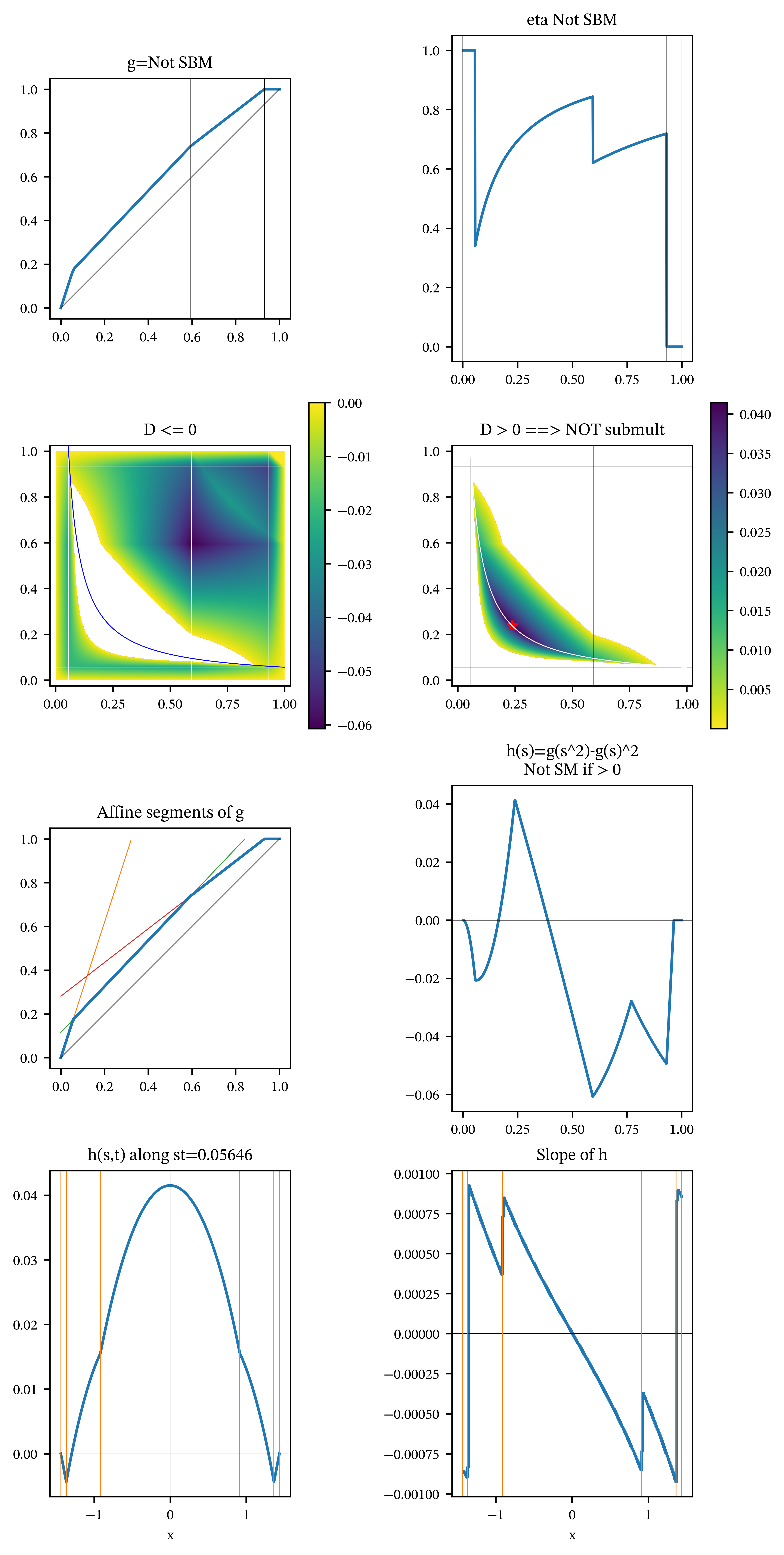
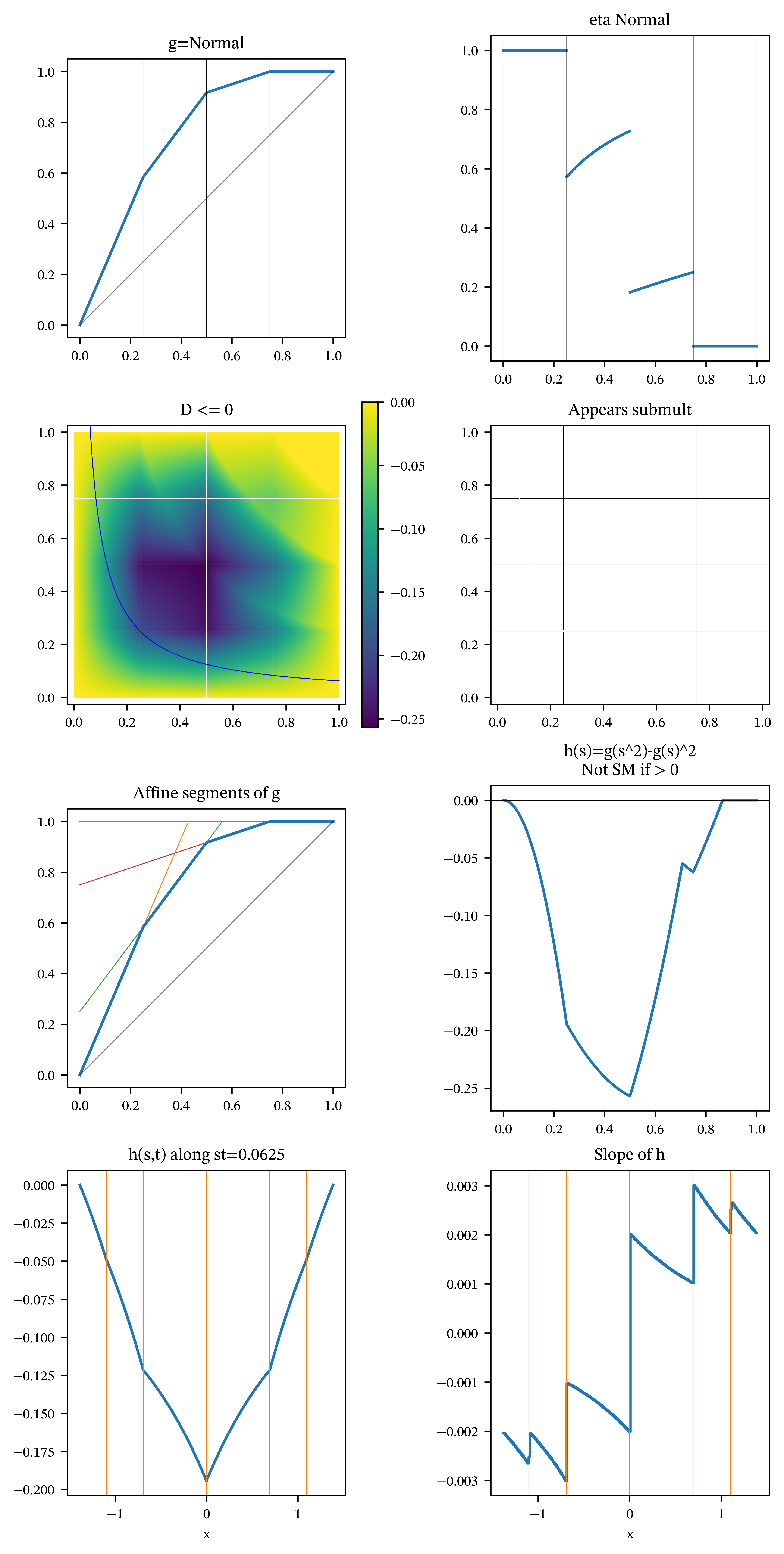
For contrast, Figure 2 shows the same information for a triTVaR that is not SBM and not DSBM, which is the usual failure mode. Figure 3 shows the most common case, where \(g\) is SBM. Observe that there are no solutions \(\eta(s)=\eta(t)\) for \(s\not= t\) (facet \((1,2)\)) and hence no interior turning points for \(h\) (confirmed in facet \((4,1)\)). You can tell this is the “generic” case because it worked for the first set of round number parameters I tried!
| s | gs | a | b | eta- | eta+ |
|---|---|---|---|---|---|
| 0.05645736 | 0.1748434 | 3.096911 | - | 1 | 0.3392686 |
| 0.5938615 | 0.7394856 | 1.050684 | 0.1155245 | 0.8437772 | 0.6201739 |
| 0.9312061 | 1 | 0.7722501 | 0.280876 | 0.719124 | - |
| 1 | 1 | - | 1 | - | - |
| s | gs | a | b | eta- | eta+ |
|---|---|---|---|---|---|
| 0.25 | 0.5833333 | 2.333333 | - | 1 | 0.5714286 |
| 0.5 | 0.9166667 | 1.333333 | 0.25 | 0.7272727 | 0.1818182 |
| 0.75 | 1 | 0.3333333 | 0.75 | 0.25 | - |
| 1 | 1 | - | 1 | - | - |
Conclusion: a happy and productive collaboration
This investigation ends with a negative result (the conjecture is false), but it is not wasted effort. The process yields:
- an exact, efficient algorithm to compute \(\max h\) for piecewise-linear distortions,
- a clear geometric picture of \([0,1]^2\) partitioned into knot regions with bilinear \(h\) on each,
- an explicit understanding of where maxima can occur:
- at knot grid points,
- at hyperbola–knot-line intersections,
- at stationary points on hyperbola arcs where \(\eta(s)=\eta(t)\),
- the hyperbola parameterization \(s=u e^x,\ t=u e^{-x}\) that makes symmetry and structure visible,
- and a practical caution: naïve Monte Carlo search can confidently return the wrong answer because the positive region of \(h\) may be extremely thin.
A final remark on the “man-machine” collaboration: the most productive part of the collaboration was a steady reduction of the problem to its essential structure, followed by an exact method to produce counterexamples. During the process, I used Gemini 3 and GPT 5.2 Thinking in “extended thinking” mode. GPT was especially helpful. It is noteworthy that GPT never over-reached. It kept reducing and saying, “If you can prove this, then…” but it never claimed a false proof.