Electrons and Spherical Harmonics
notes
science
mathematics
llm
elements
1 TL;DR
Chatters and I have been learning about electrons and elements.
Energy level = shell = principal quantum number \(n\)
Sub-shell = {orbitals} with the same \(n\) and angular momentum \(\ell\) (labeled s, p, d, f etc.)
Configuration determined by \((n, \ell, m_l, m_s)\)
Orbitals not orbits to remind you they are not like planetary orbits. It is a wave function whose squared modulus gives an occupancy density.
Each orbital is one spatial wave function. It can can contain up to 2 electrons (arrows in boxes, one up and one down).
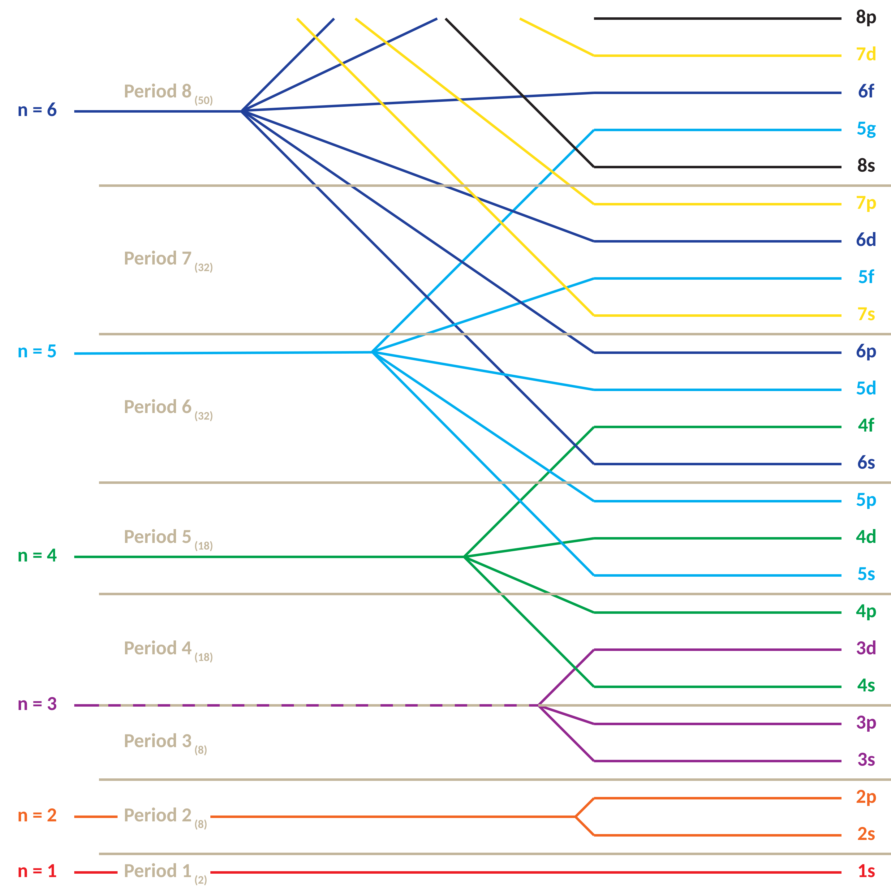
Aufbau principle: order by \(n+\ell\) and descending \(n\)
Hund’s rule: orbitals are filled singly before doubly
2p: ↑  ↑  ↑     → 3 orbitals filled singly
2p: ↑↓ ↑  ↑     → second electron paired in first orbital
Pauli exclusion (\(m_s=1/2,\ -1/2\)).
Spherical harmonics describe the angular part, \(Y_{\ell m}(\theta, \phi)\). They are:
- Solutions to the angular part of the Laplacian (or Schrödinger equation) in spherical coordinates.
- Depends only on \(\ell\) and \(m\)
- Functions on the unit sphere \(S^2\)
- Used in many contexts: quantum mechanics, classical wave equations, gravitational fields, etc.
Radial solution \(R_{n\ell}(r)\) – Comes from solving the radial Schrödinger equation for a given potential – Depends on energy level \(n\) and angular momentum \(\ell\)
2 Remember
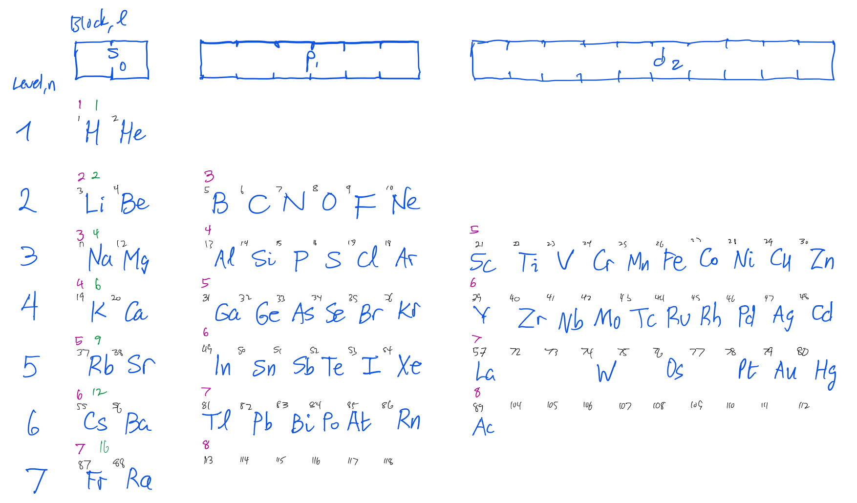
Figure 1 shows the more memorable part of the periodic table, with rows corresponding to levels. The blocks snake down 1s, 2s, 2p, 3s, 3p, 4s, 3d, 4p, 5s, 4d, 5p, 6s, 4f, 5d, 6p, 7p, 8s (no elements there yet).
3 Quantum Numbers and Orbital Naming
An orbital is a single wave function \(\psi_{n\ell m}\). Orbitals are also called sub-shells. It describes the state of one electron and is specified by three quantum numbers \(n\), \(\ell\), and \(m\). There are \(2\ell + 1\) orbitals in a given subshell (one per \(m\)). Each orbital can hold 2 electrons (spin up/down). A subshell is a set of orbitals with the same \(n\) and \(\ell\). They are grouped by letter: s, p, d, f, etc. and contain all orbitals with different \(m\) values for a given \(\ell\). For examples, \((n=1, \ell=0)\) → 1s, \((n=2, \ell=1, m=0)\) → 2p (m=0), and \((n=3, \ell=2)\) → 3d. Each \((n, \ell)\) subshell contains \(2(2\ell + 1)\) electrons: 2 per orbital (spin up/down).
| Symbol | Name of Quantum Number | Values | Meaning |
|---|---|---|---|
| \(n\) | Principal | \(1, 2, 3, \dots\) | Energy level (“shell”) |
| \(\ell\) | Azimuthal or Orbital angular momentum | \(0, 1, \dots, n-1\) | Subshell (“s”, “p”, “d”, …) |
| \(m_l\) | Orbital magnetic | \(-\ell, \dots, \ell\) | Orientation of orbital |
| \(m_s\) | Spin magnetic | \(-1/2,\ 1/2\) | \(z\) component of spin ang mo |
Orbitals were discovered because the spectral lines of shells split into different energy levels. The lowest energy of 4, 4s, is lower than the highest 3d. The names come from spectroscopic observations of atomic emission lines, well before quantum mechanics was developed. They describe groups of spectral lines seen in early atomic spectroscopy (especially alkali metals).
| \(\ell\) | Label | Stands for | Spectral meaning |
|---|---|---|---|
| 0 | s | sharp | Narrow, well-defined lines |
| 1 | p | principal | Strong lines in the main series |
| 2 | d | diffuse | Broader, more complex lines |
| 3 | f | fundamental | Least structured, lowest energy in IR |
| 4+ | g, h, … (rarely used) | beyond f, continue alphabetically |
| \(n\) | Subshells | Max Electrons | Cumulative |
|---|---|---|---|
| 1 | 1s | 2 | 2 |
| 2 | 2s, 2p | 8 | 10 |
| 3 | 3s, 3p, 3d | 18 | 28 |
| 4 | 4s, 4p, 4d, 4f | 32 | 60 |
| 5 | 5s, 5p, 5d, 5f | 32 | 92 |
| 6 | 6s, 6p, 6d, 6f | 32 |
4 Hydrogen Wavefunctions and Factorization
The time-independent wave function of a hydrogen orbital factorizes as: \[ \psi_{n\ell m}(r, \theta, \phi) = R_{n\ell}(r) \cdot Y_{\ell m}(\theta, \phi). \]
The first part, \(R_{n\ell}(r)\) is a real-valued radial function. The radial probability density \[ P(r) = r^2 |R(r)|^2 \] shows the probability of finding the electron between \(r\) and \(r+dr\), regardless of direction. It includes the Jacobian \(r^2\) from spherical coordinates. It is plotted in 1D radial plots in Section 6. It answers: “How far from the nucleus is the electron likely to be?”
The second part, \(Y_{\ell m}(\theta, \phi)\) is a complex-valued spherical harmonic function. The angular probability \[ |Y_{\ell m}(\theta, \phi)|^2 \] gives the density over directions on the shell at radius \(r\). For example, \(|Y_{10}|^2 \propto \cos^2 \theta\) is highest at the poles, and zero at the equator. It defines the shape of the “cloud”: lobes, nodal planes, etc.
The full probability density is \[ |\psi|^2 = |R(r)|^2 \cdot |Y_{\ell m}(\theta, \phi)|^2 \] This factorization holds because the Coulomb potential is spherically symmetric. The full probability of finding the electron in a small volume element is: \[ |\psi(r, \theta, \phi)|^2\, r^2 \sin\theta\, dr\, d\theta\, d\phi = |R(r)|^2\, r^2\, dr \cdot |Y_{\ell m}(\theta, \phi)|^2 \sin\theta\, d\theta\, d\phi \] That is:
- \(r^2 |R(r)|^2, dr\): total probability in a thin shell at distance \(r\)
- \(|Y_{\ell m}(\theta, \phi)|^2, d\Omega\): distributes that probability across angles on the shell
The radial probability density tells you how far the electron tends to be. The angular part tells you where on that shell.
Factorization holds because:
- The hydrogen potential is central (depends only on \(r\)).
- The time-independent Schrödinger equation is separable in spherical coordinates.
It breaks down if:
- The potential isn’t spherically symmetric (e.g. in multi-electron atoms or molecules).
- You have a superposition of eigenstates (which reintroduces time dependence and interference).
- You’re including external fields (e.g. Zeeman, Stark).
The orbitals can be visualized using the factorization.
- Radial plots: show \(P(r)\) vs. \(r\)
- Angular plots: plot \(|Y_{\ell m}|^2\) on the sphere
- Electron clouds (point clouds): sample from \(|\psi|^2\) to show spatial structure
These visualization complement each other. The point cloud reveals everything: you see both shell structure (radial) and lobe shape (angular).
5 Angular structure is set by \(\ell\) and \(m\)
The spherical harmonic \(Y_{\ell m}(\theta, \phi)\) defines the angular part of the wave function. It determines the directional distribution on the unit sphere.
| \(\ell\) | \(m\) values | Angular structure |
|---|---|---|
| 0 | 0 | Constant → spherical symmetry |
| 1 | −1, 0, +1 | Dumbbell lobes (p orbitals) |
| 2 | −2 to +2 | Cloverleaf, toroidal shapes (d orbitals) |
| … | … | Increasing angular complexity |
When \(\ell = 0\), the only allowed \(m=0\), and: \[ Y_{00}(\theta, \phi) = \frac{1}{\sqrt{4\pi}} \quad \text{(constant)} \] → complete spherical symmetry: \[ |\psi(r, \theta, \phi)|^2 = |R_{n0}(r)|^2 \cdot \underbrace{|Y_{00}|^2}_{\text{constant}}. \] Because \(Y_{00}\) is constant, the cloud looks like concentric fuzzy spheres. There is no angular dependence—all directions are equally likely. The cloud is perfectly symmetric about the origin
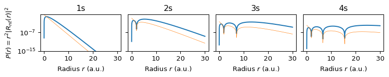
The radial structure is set by \(n\) and \(\ell\). The function \(R_{n\ell}(r)\) describes how the amplitude changes with radius. The radial probability density is: \[ P(r) = r^2 |R_{n\ell}(r)|^2. \] This shows where the electron is likely to be, in terms of distance from the nucleus. As \(n\) increases: The number of radial nodes increases (\(n -\ell - 1\)) and the distribution becomes more multi-modal. In fact, the radial function \(R_{n0}(r)\) has \(n - 1\) nodes, so \(1s\) has no nodes, \(2s\) has 1 radial node (two concentric shells), \(3s\) has 2 radial nodes (three shells). The radial probability density: \[ P(r) = r^2 |R_{n0}(r)|^2 \] is n-modal (one peak per radial region separated by nodes), se Section 6.
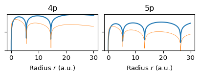
6 Radial Probability Densities by \(n\) and \(\ell\)
Compare graphs of Hydrogen radial probabilities
6.1 \(\ell=s\) Orbitals
6.2 \(\ell=p\) Orbitals
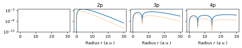
6.3 \(\ell=d\) Orbitals
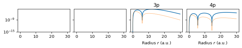
6.4 \(\ell=f\) Orbitals
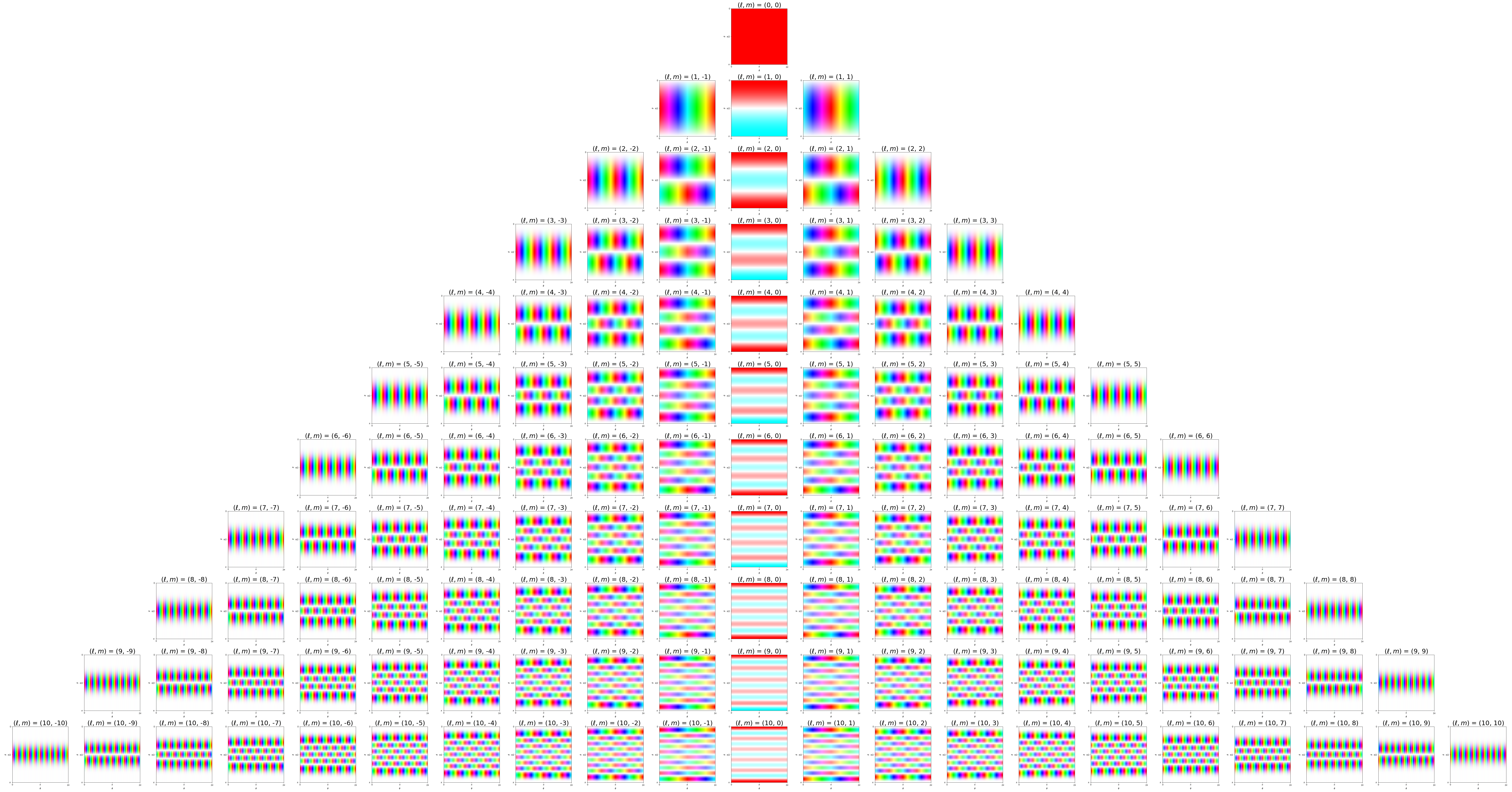
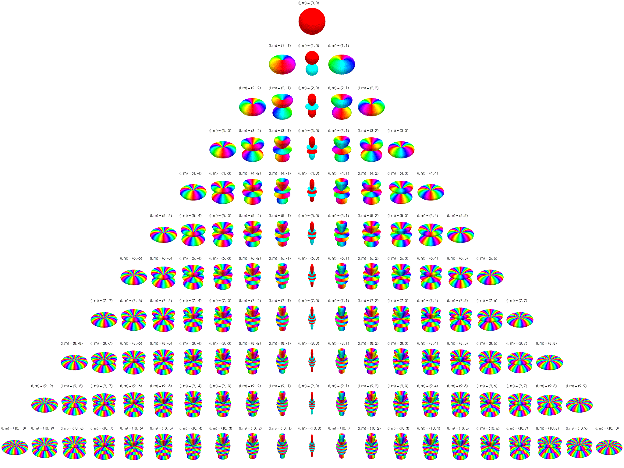
7 Visualization of complex spherical harmonics
Source: Wikipedia Twistar48 - Own work, CC BY-SA 4.0, Attribution.
7.1 2D polar/azimuthal angle maps
Below the complex spherical harmonics are represented on 2D plots with the azimuthal angle, \(\phi\), on the horizontal axis and the polar angle, \(\theta\), on the vertical axis. The saturation of the color at any point represents the magnitude of the spherical harmonic and the hue represents the phase.
The nodal ‘line of latitude’ are visible as horizontal white lines. The nodal ‘line of longitude’ are visible as vertical white lines.
7.2 Polar plots
Below the complex spherical harmonics are represented on polar plots. The magnitude of the spherical harmonic at particular polar and azimuthal angles is represented by the saturation of the color at that point and the phase is represented by the hue at that point.
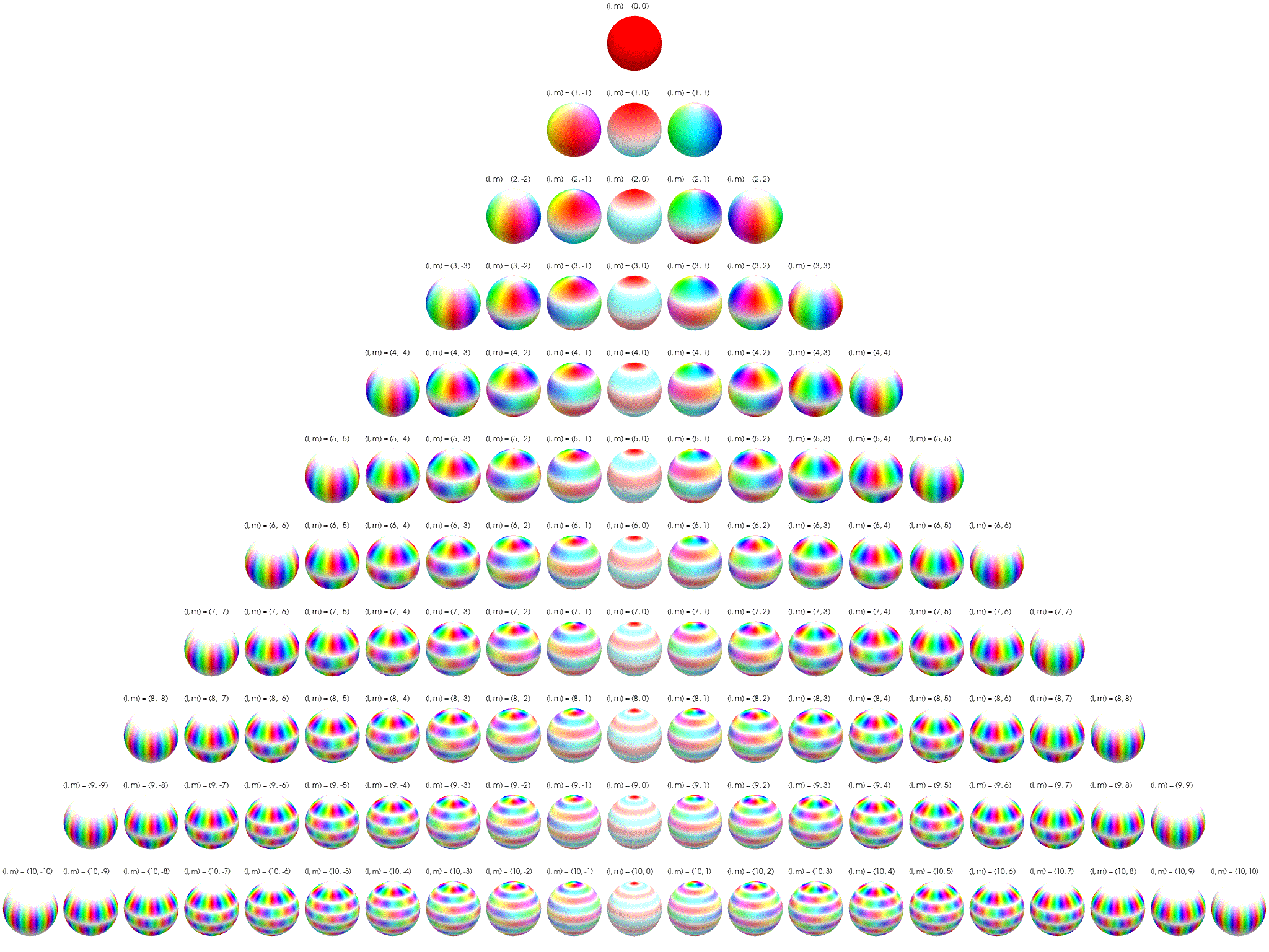
7.3 Polar plots with magnitude as radius
Below the complex spherical harmonics are represented on polar plots. The magnitude of the spherical harmonic at particular polar and azimuthal angles is represented by the radius of the plot at that point and the phase is represented by the hue at that point.
7.4 Electron cloud examples
These plots show simulated electron positions.
8 Ionization Energy

Ionization energy increases across a period and decreases down a group in the periodic table. As atomic number increases, the nuclear charge grows, pulling electrons more tightly and raising the energy required to remove one. However, this trend is modulated by the shell structure of electrons. Electrons in higher principal quantum number shells (larger \(n\)) are farther from the nucleus and more shielded by inner electrons, reducing their binding energy. As a result, ionization energy drops sharply at the start of a new shell. Sharp peaks occur at noble gases due to their closed-shell configurations, which are especially stable and energetically costly to disrupt.
Zinc (Zn), cadmium (Cd), and mercury (Hg) each terminate a filled \(d^{10}s^2\) configuration, with the outermost electrons in a fully occupied \(s\)-orbital sitting atop a compact, closed \(d\)-shell. These configurations are unusually stable, and the \(d\)-electrons do a poor job of shielding the outer \(s\)-electrons. As a result, the first ionization energies of these elements are relatively high, especially in mercury, where relativistic effects contract the 6s orbital further, strengthening the nuclear attraction.
Gallium (Ga) and indium (In) follow filled \(d^{10}\) shells and begin populating the \(p\)-subshell. The newly added \(p^1\) electron is loosely held because the inner \(d\)-electrons shield poorly and the \(p\)-orbital is more diffuse. This causes a marked drop in ionization energy compared to aluminum or boron, despite a higher nuclear charge. The result is a noticeable dip in the ionization energy trend that reflects the structural discontinuity between filled \(d\)-shells and new \(p\)-electron occupation.
Gadolinium (Gd) shows a noticeable bump in ionization energy within the lanthanide series. Its configuration includes a half-filled 4f⁷ shell and a single 5d electron. Half-filled subshells are especially stable due to exchange energy, and the 5d electron is relatively well bound. As a result, removing this electron requires more energy than for neighboring elements, leading to a locally elevated ionization energy.
Lutetium (Lu), by contrast, has a fully filled 4f¹⁴ shell and a single 5d electron, yet its ionization energy is slightly lower than expected. The 5d electron is farther from the nucleus and experiences less shielding from the compact 4f electrons, making it easier to remove. Despite the closed 4f shell, this outer 5d¹ electron is relatively weakly bound, causing a small dip at the end of the lanthanide trend.
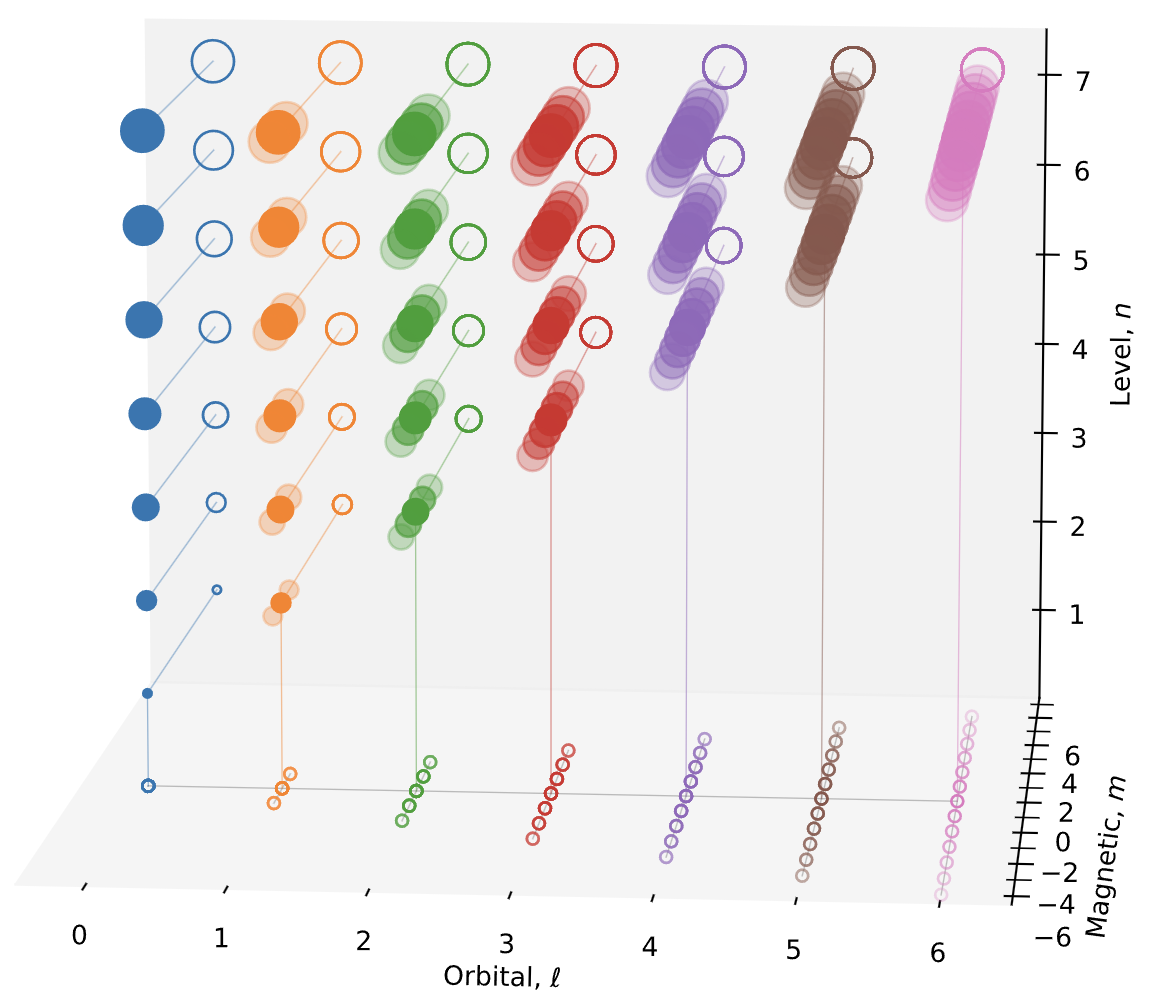
9 Elements arranged by principal and orbital quantum numbers \((\ell, n)\)

Figure 7 shows the elements by the location of its last electron added, see Section 9.1 for how this is determined. The figure illustrates that \(s\) orbitals hold two electrons (\(m = 0\), spin up and down), \(p\) orbitals six (\(m = -1, 0, 1\)), \(d\) ten, and \(f\) fourteen, each with paired spins. Energy levels are filled in order of increasing \(n + \ell\), with ties resolved by lower \(n\). Figure 8 shows the same data transformed so that energy ordering (by \(n + \ell\)) appears vertical. The superscripts reflect that electrons are placed one per orbital (Hund’s rule) before spin-pairing.
Detailed table Wikipedia
9.1 Last electron added
The last electron need not be the outermost, i.e., the highest-energy occupied \((n, \ell, m)\) state, because the Aufbau filling order incorporates:
- Aufbau principle (lowest energy levels first),
- Pauli exclusion (one per \((n, \ell, m, s)\)),
- Hund’s rule (maximize spin multiplicity / spread across m first),
- Energy subshell ordering (e.g., \(4s\) before \(3d\)).
Some subshells (like 5s, 4d) may be increased simultaneously. The first time two orbitals increase simultaneously occurs between rhodium (Rh, Z=45) and palladium (Pd, Z=46), where both the 4d and 5s subshells are involved. While Rh has a configuration ending in 5s1 4d8, Pd has a closed 4d10 configuration and no 5s electron. This means that from Rh to Pd, one electron is added to the 4d subshell and one is removed from the 5s subshell—two changes happening at once. A diff-based method, which only compares the electron counts in each orbital between successive configurations, cannot reliably determine where the last electron went in such cases. To solve this problem, we use a simulated Aufbau filling approach, where electrons are added one at a time according to physical principles, regardless of how the configuration string is written. Other examples of dual orbital changes include Cr (3d5 4s1) following V (3d3 4s2), Mo (4d5 5s1) following Nb (4d4 5s1), and Pt (5d9 6s1) following Ir (5d7 6s2). These irregular cases often involve subshell rearrangements driven by exchange energy or relativistic effects.
To determine where the last electron went, we build a list of orbitals in canonical energy-filling order and simulate placing electrons one at a time. This guarantees you know exactly where the final electron went for each element. Step-by-step:
Define the Aufbau filling order using
(n, ℓ)tuples:[ (1, 0), # 1s (2, 0), (2, 1), (3, 0), (3, 1), (4, 0), (3, 2), (4, 1), (5, 0), (4, 2), (5, 1), (6, 0), (4, 3), (5, 2), (6, 1), (7, 0), (5, 3), (6, 2), (7, 1), (6, 3), (7, 2), (7, 3) ]For each element:
- Fill each orbital using its allowed capacity \(2(2\ell + 1)\)
- Keep track of how many electrons you’ve added
- When you reach the element’s atomic number, record the last orbital filled
Use Hund’s rule to determine \(m\): spread across allowed \(m\)-values cyclically
9.2 Transformed plot against \(n+\ell\)
Figure 8 plots \(\ell\) against \(n+\ell\) which better corresponding to the energy level.

10 Anomalous configurations up to uranium
Table 1 is a list of anomalous electron configurations up to uranium (Z = 92), where elements deviate from the naïve Aufbau order. The most well-known and agreed-on anomalies are Cr, Cu, Mo, Pd, Ag, Pt, Au In the actinides, starting around Ac to U, the boundaries between 5f and 6d are fuzzy. Some configurations differ across sources (textbooks, experiments, computations); for example, some give Ac as 7s² 6d¹, others as 7s² 5f¹. Pd is double anomalous, with no 5s.
| Element | Z | Expected Ending | Actual Ending | Why it’s a surprise |
|---|---|---|---|---|
| Cr | 24 | 4s² 3d⁴ | 4s¹ 3d⁵ | Half-filled d⁵ is more stable (exchange energy) |
| Cu | 29 | 4s² 3d⁹ | 4s¹ 3d¹⁰ | Full d¹⁰ subshell is favored over 4s² |
| Nb | 41 | 5s² 4d³ | 5s¹ 4d⁴ | Exchange energy gain from more unpaired d electrons |
| Mo | 42 | 5s² 4d⁴ | 5s¹ 4d⁵ | Half-filled d⁵ again preferred |
| Ru | 44 | 5s² 4d⁶ | 5s¹ 4d⁷ | Unusual stability pattern; 5s electron is promoted |
| Rh | 45 | 5s² 4d⁷ | 5s¹ 4d⁸ | Similar to Ru; favors d over s |
| Pd | 46 | 5s² 4d⁸ | 4d¹⁰ (no 5s) | Very rare case: fully fills d, no s electron present |
| Ag | 47 | 5s² 4d⁹ | 5s¹ 4d¹⁰ | Like Cu, full d¹⁰ is preferred |
| Pt | 78 | 6s² 5d⁸ | 6s¹ 5d⁹ | Exchange and relativistic effects stabilize 5d⁹ |
| Au | 79 | 6s² 5d⁹ | 6s¹ 5d¹⁰ | Full 5d shell again preferred (relativistic) |
| Ac | 89 | 7s² 6d¹ | (As expected) | But sometimes written with 5f¹ → classification ambiguity |
| Th | 90 | 7s² 6d² | (As expected) | But 5f sometimes starts here instead |
| Pa | 91 | 7s² 6d¹ 5f² | (Ordering varies) | Mixed d/f filling: order hard to define cleanly |
| U | 92 | 7s² 6d¹ 5f³ | (As expected) | But distribution among 5f and 6d varies in texts |
11 Elements in \((n,\ell, m)\)-space
The set of possible \((n,\ell, m)\) forms an irregular tetrahedron. For (spherically symmetric H), the projection to \((n, \ell)\) defines the radial distribution and \((\ell, m)\) the angular distribution. For a given \(\ell\), as \(n\) increases the radial distribution becomes more multi-modal and thicker tailed.

12 Periodic table
| Period | \(s\) | \(p\) | \(d\) | \(f\) | Sum | Cumsum | Noble |
|---|---|---|---|---|---|---|---|
| 1 | 2 (1s) | 2 | 2 | He | |||
| 2 | 2 (2s) | 6 (2p) | 8 | 10 | Ne | ||
| 3 | 2 (3s) | 6 (3p) | 8 | 18 | Ar | ||
| 4 | 2 (4s) | 6 (4p) | 10 (3d) | 18 | 36 | Kr | |
| 5 | 2 (5s) | 6 (5p) | 10 (4d) | 18 | 54 | Xe | |
| 6 | 2 (6s) | 6 (6p) | 10 (5d) | 14 (4f) | 32 | 86 | Ra |
| 7 | 2 (7s) | 6 (7p) | 10 (6d) | 14 (5f) | 32 | 118 | Og |
For a discussion of Madelung’s (aufbau) rule and its apparent contradictions (added vs ionized electrons) see Electron configuration and aufbau principle.
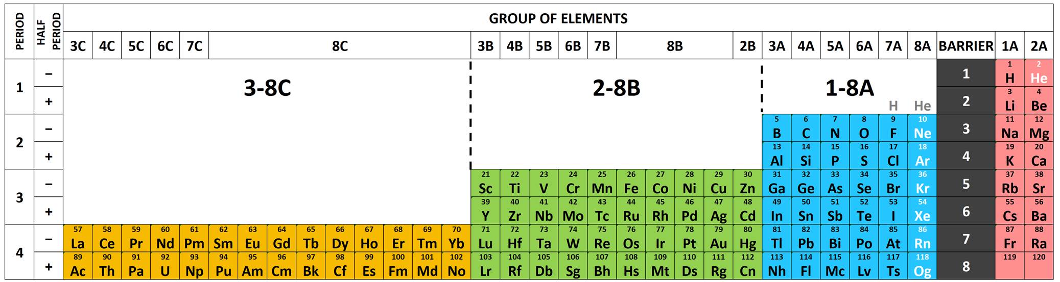

Sciencegeek has a page with many different periodic tables, including the basis for this spreadsheet-based version.
![From spreadsheet C:/Users/steve/S/TELOS/Spreadsheets/[periodic-table.xlsx]PeriodicTable (hacked)](img/pt.png)