Code
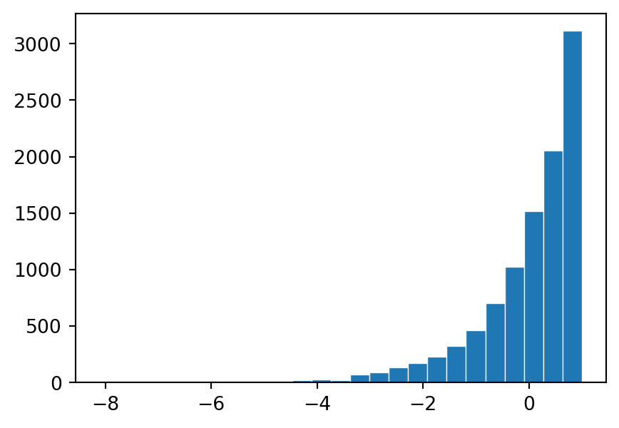
print(f'Sample mean at t={ts[-1]:.3f} equals {np.mean(M[:,-1]):.4f} vs. expected 0.0.')Sample mean at t=9.111 equals 0.0009 vs. expected 0.0.
Given an exponential random variable \(T\) with the hazard function \(\alpha(t) = t\), the compensator \(A_t\) is defined as \(A_t = \min(t, T)\). Observe that \(N_t\) is either 0 or 1, where \(N_t = 1\) if \(t \geq T(\omega)\) and 0 otherwise. This setup defines a one-point process \(N_t\).
The compensator \(A_t\) is designed to make \(N_t - A_t\) a martingale. To understand why \(N_t - A_t\) is a martingale, recall the definition: a process \(M_t\) is a martingale with respect to a filtration \(\mathcal{F}_t\) if for all \(s \leq t\), \(\mathsf{E}[M_t | \mathcal{F}_s] = M_s\).
Here’s the intuition behind \(N_t - A_t\) being a martingale:
In essence, the compensator \(A_t\) “anticipates” the jump of \(N_t\) such that the expected increment in \(N_t - A_t\) given the past (up to \(s < t\)) is zero, which is the martingale property. This balancing act makes \(N_t - A_t\) a martingale.
Understanding \(N_t - A_t\) using an infinitesimal time period \(dt\) is quite insightful and aligns with the intuition behind stochastic calculus, particularly in the context of martingales. For \(t<T\):
When \(t\ge T\) there are no further changes in \(N\) or \(A\).
This reasoning aligns with the continuous-time martingale theory and provides a solid foundation for understanding why \(N_t - A_t\) behaves as a martingale, despite the non-intuitive appearance of its paths.
The key to understanding why \(N_t - A_t\) is a martingale despite its appearance (lines with a slope -1 getting more and more negative) lies in the definition of a martingale and the conditional expectation.
A martingale doesn’t necessarily have to “look” like it has no drift along a single path. Instead, the requirement is that the expected future value across all paths, given all past information, is equal to the current value. This is a probabilistic statement about expectations, not a deterministic one about the paths themselves.
For \(N_t - A_t\), here’s what’s happening:
The essence of the martingale property here is that the compensator \(A_t\) is designed to account for the “average” behavior of \(N_t\). While individual paths of \(N_t - A_t\) may appear to have a drift, when you condition on the past information, the expected change in \(N_t - A_t\) averaged over all paths is zero, which is the core of the martingale definition.
If you simulate and plot multiple realization paths of \(N_t - A_t\), you see a variety of behaviors. Some paths would have the jump in \(N_t\) occurring early (before \(t = 1\)), resulting in \(N_t - A_t\) being positive for a significant portion of the time afterward. Other paths might have the jump occurring much later, resulting in \(N_t - A_t\) being negative right up until the jump happens.
However, the key point is that when you take the average of many such paths at any fixed future time \(t\), the positive and negative deviations cancel out, leading to an average value of zero—the starting value. A similar argument applies to changes from a future time \(s\). This aligns with the definition of a martingale: the expected value of \(N_t - A_t\) at any future time, given the past, is equal to its current value, which is zero at the start.
While individual paths might show significant up or down deviations, the “average path” when considering a large number of simulations would hover around zero, reflecting the martingale property that the expected change in \(N_t - A_t\), conditioned on the past, is zero at any point in time.
import matplotlib.pyplot as plt
import numpy as np
import scipy.stats as ss

fz = ss.expon()

# failure times
T = fz.rvs((10000, 1))

# sampling times
ts = np.linspace(0, np.max(T), 101)

# individual paths
paths = np.where(T > ts, 0, 1)

# compensated process
M = paths - np.minimum(ts, T)

fig0, ax0 = plt.subplots(1, 1, figsize=(5, 3.5))
fig1, ax1 = plt.subplots(1, 1, figsize=(5, 3.5))

for v in M[:2500]:
    ax0.plot(ts, v, lw=.5, c='C0', alpha=.05)

ax1.hist(M[:, -1], bins=25, lw=.5, ec='w');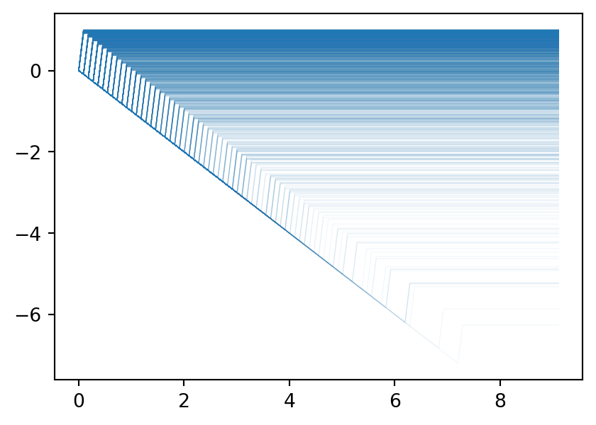
Note:
print(f'Sample mean at t={ts[-1]:.3f} equals {np.mean(M[:,-1]):.4f} vs. expected 0.0.')Sample mean at t=9.111 equals 0.0009 vs. expected 0.0.