Conditional Expectations Given The Sum of Independent Random Variables with Regularly Varying Densities

notes

Summary of results and examples from a recent paper of Denuit et al.

Author

Stephen J. Mildenhall

Published

2024-04-04

This post summarizes results from the recent paper [1].

Assumptions

$X$ and $Y$ are independent random variables with regularly varying densities, $f(x)=x^{-\alpha}L(x)$ for slowly varying $L$. The tail indices are $\alpha_X$ and $\alpha_Y$. Assume $\min(\alpha_X, \alpha_Y) >2$ so that $X$ and $Y$ have finite expectations.

$S=X+Y$, $m_X(s)=\mathsf E[X\mid S=s]$, and $m_Y(s)=\mathsf E[Y\mid S=s]$.

In all these examples $\alpha_Y \le \alpha_X$, meaning that $Y$ is thicker tailed than $X$.

Findings

Proposition 2.3.: If $f_Y$ is ultimately decreasing and $f_X$ is ultimately small compared to $f_{X+Y}$ then $\lim_s\inf m_X(s)\ge \mathsf E[X]$
Property 3.1.: If $\alpha_Y \le \alpha_X$ then $m_Y(s)\to\infty$ as $s\to\infty$, meaning the thicker tailed projection always tends to infinity.
Property 3.2.: If $\alpha_X > \alpha_Y + 1$ then $m_X(s) \to \mathsf E[X]$ as $s\to\infty$.
Property 3.3.: In the case 3.2, there is a non-empty interval in $(0, \infty)$ where $m_X$ is decreasing.
Property 3.5.: If second moments exist then $\mathsf{cov}(m_X(S), m_Y(S))\ge 0$.

Property 3.5 means that “if there are values for which the monotonicity of $m_X(·)$ and $m_Y(·)$ differ, those must be values with small probability of occurrence or with slight differences in the increasing/decreasing rate, as in overall terms the dependence remains positive.”

Property 3.6.: If $\alpha_X > 2$ and $\alpha_Y \le \alpha_X < \alpha_Y + 1$ then $m_X(s) \to \infty$ as $s\to\infty$.
Property 3.9.: If $\alpha_X = \alpha_Y + 1$ then

If $L_X(s)/L_Y(s)\to\infty$ as $s\to\infty$ then $m_X(s)\to\infty$ as $s\to\infty$.
If $L_X(s)/L_Y(s) = k$ as $s\to\infty$ then $m_X(s)\to\mathsf E[X] + k$ as $s\to\infty$.

In the case 3.9, $m_X$ can be increasing.

Asymptotic Expansions

Section 4 gives asymptotic expansions for $m_X$ in the corresponding cases.

Property 4.3.: If $\alpha_X > \alpha_Y + 2$ then \[m_x(s) \sim \mu_X+\frac{\alpha_Y}{s}\mathsf{Var}(X).\]
Property 4.5.: If $\alpha_Y + 2 > \alpha_X > \alpha_Y+1$ then \[m_x(s) \sim \mu_X+s \frac{f_X(s)}{f_X(s)}.\]
Property 4.7.: If _Y + 1 > _X > _Y$ then

If $\alpha_X\in(\alpha_Y+1/2, \alpha_Y+1)$ then \[m_x(s) \sim s \frac{f_X}{f_X}\left( 1 + \mu_X\frac{f_Y}{sf_X} - \frac{f_X}{f_Y} \right).\]
If $\alpha_X\in(\alpha_Y+1/3, \alpha_Y+1/2)$ then \[m_x(s) \sim s \frac{f_X}{f_X}\left( 1 - \frac{f_X}{f_Y} +\mu_X\frac{f_Y}{sf_X} \right).\]
If $\alpha_X\in(\alpha_Y, \alpha_Y+1/3)$ then \[m_x(s) \sim s \frac{f_X}{f_X}\left( 1 - \frac{f_X}{f_Y}\left(1 - \frac{f_X}{f_Y}\right) \right).\]

Property 4.9.: If $\alpha_Y = \alpha_X=\alpha$ and $f_X\sim cf_Y$, then \[m_X(s)\sim \frac{c}{1+c}s\left(1+ \frac{1}{s}\left(\frac{\alpha}{1+c}(\mu_Y-\mu_X) + \frac{\mu_X}{c} - \mu_Y \right)\right).\]

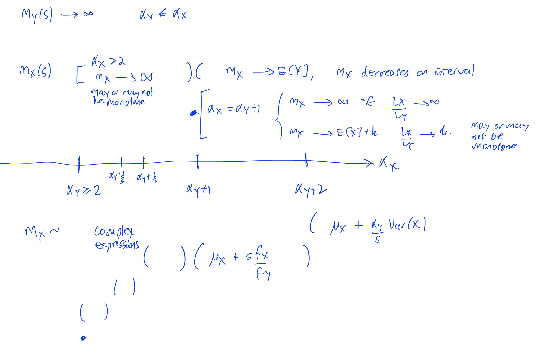
The next figure lays out the various possible options.

Schematic of the different possible behaviors of m_X(s). — Schematic of the different possible behaviors of $m_X(s)$.

Examples

The paper provides examples for all the behaviors described by the different properties. It uses a parameterizations in terms of $\alpha$ for clarity.

The examples below use aggregate with scipy.stats parameterization to illustrate the same behaviors.

Code to setup .

Code

import numpy as np
from aggregate import build, knobble_fonts
knobble_fonts(True)

def example(aX, aY, lam, scale, mm, verbose):
    k = lam ** (aX - aY) * aX / aY
    port = build('port P '
                f'agg X 1 claim sev {lam} * pareto {aX} - {lam} fixed '
                f'agg Y 1 claim sev {lam} * pareto {aY} - {lam} fixed '
                , normalize=False, log2=20, recommend_p=1-1e-13)
    if verbose:
        qd(port)
        # port.plot()

    l = port.q(0.999) * scale
    ax = port.density_df.loc[:l].filter(regex='exeqa_[XYt]').plot(figsize=(3,3))
    ax.axhline(port.X.est_m, c='k', lw=.5, label=f'Mean X {port.X.est_m:.2f}')
    if aY + 1 == aX:
        ax.axhline(port.X.est_m + k, c='r', lw=.5, label=f'Mean X + k {k + port.X.est_m:.2f}')
    ax.set(ylim=[0, l], xlim=[0,l])
    # add asymptotic estimates
    s = np.array(port.density_df.loc[:l].index)
    fx = port.X.density_df.loc[:l].p_total
    fy = port.Y.density_df.loc[:l].p_total
    mx = port.X.agg_m
    sx = port.X.agg_var
    appx = None
    fxy = fx / fy
    if aX > aY + 2:
        if verbose: print('more than 2')
        appx = mx + aY * sx / s
    elif aY + 2 > aX > aY + 1:
        if verbose: print('more than 1')
        appx = mx + s * fxy
    elif aY + 1 > aX > aY + 0.5:
        if verbose: print('more than 0.5')
        appx = s * fxy  * (1 + mx * fy / fx / s - fxy)
    elif aY + 0.5 > aX > aY + 1/3:
        if verbose: print('more than 1/3')
        appx = s * fxy  * (1 - fxy + mx * fy / fx / s)
    elif aX < aY + 1/3:
        if verbose: print('less than 1/3')
        appx = s * fxy  * (1 - fxy + fxy**2)
    if appx is not None:
        ax.plot(s, appx, ls='--', lw=1, label='Asymptotic expansion')
    ax.legend()
    ax.set(title=f'αX={aX}, αY={aY}, λ={lam}')
    if aX > aY + 1:
        ax.set(ylim=[0, mm * port.X.est_m])
    else:
        ax.set(aspect='equal')

Here are some examples.

for aX, aY, lam, scale, mm in zip(
    [5.5, 4.5, 4.0, 3.75,  3.4, 3.25],
    [3.0, 3.0, 3.0,  3.0,  3.0, 3.0],
    [100, 100, 100, 100, 100, 100],
    [10, 15, 2, 2, 7.5, 100],
    [5, 5, 2.5, 1, 1, 1]
):
    example(aX, aY, lam, scale=scale, mm=mm, verbose=False)

(a) Tails differ by 2.5, humped behavior tending to mean of $X$.

An especially interesting example is the case with equal indices where you can have a humped distribution that still tends to infinity.

# Example 4.10
a = 7
l = 2
d = l
c = (a - 1) / l
scx = 1
scy = 2

port = build('port T '
            f'agg X 1 claim sev {scx} * burr12 {c} {d} fixed '
            f'agg Y 1 claim sev {scy} * burr12 {c} {d} fixed '
            , log2=19, bs=1/256, normalize=False, padding=2 )
d = 15

ax = port.density_df.filter(regex='exeqa_[XYt]').plot(
 xlim=[0, 100], ylim=[0, 100], figsize=(4,4))
ax.axhline(1.35, lw=.5)
xs = port.density_df.loss.values
cc = (scx / scy) ** (a-1)
mx = port.X.agg_m
my = port.Y.agg_m
appx = cc / (1+cc) * xs * (1 + 1/xs * (a / (1+cc)*(my - mx) + mx/cc - my ))
ax.plot(xs, appx, lw=.5, ls=':', label='Approx')
ax.legend(loc='upper left');

# zoomed version
ax = port.density_df.filter(regex='exeqa_[XYt]').plot(
 xlim=[0, 100], ylim=[0, 2.5], figsize=(4,4))
ax.axhline(1.35, lw=.5)
ax.plot(xs, appx, lw=.5, ls=':', label='Approx')
ax.legend(loc='lower right');

Extensions

Section 5 extends sections 3 and 4 to the case of zero-augmented variables.

Section 6 considers sums of more than two variables. If the gap between the smallest smallest $\alpha$ and the rest is more than 1 then $m_i(s)\to\mathsf E[X_i]$ for all but the thickest tailed distribution (Proposition 6.2).

References

Denuit, M., Ortega-jimenez, P., Robert, C.Y.: Conditional Expectations Given The Sum Of Independent Random Variables With Regularly Varying Densities, https://dial.uclouvain.be/pr/boreal/object/boreal%3A285506/datastream/PDF_01/view, (2024)