Academic Descriptions of Risk
Academic Descriptions of Risk
Eeckhoudt and Schlesinger (2006)
Equal probability lotteries \([a, b]\) describe outcomes \(a\) and \(b\), which can be fixed or random.
\(k>0\) wealth level
\(\epsilon\) zero-mean random variable, independent of any other random variables that may be present in an individual’s initial wealth allocation.
Equal-probability lotteries.
Monotonic: (more to less) \([0,0] \succeq [-k -k]\)
Risk averse: \([0,0] \succeq [\epsilon, \epsilon]\)
Prudence: \([-k, \epsilon] \succeq [0, \epsilon - k]\)
If preferences are also monotonic and risk averse, the individual prefers to receive one of the two “harms” for certain, with the only uncertainty being about which one is received, as opposed to a 50-50 chance of receiving both “harms” simultaneously or receiving neither. Borrowing terminology from Kimball (1993), the above property implies that \(-k\) and \(\epsilon\) are “mutually aggravating” for all initial wealth levels \(x\) and for all \(k\) and all \(\epsilon\).
We also can interpret prudence as type of “location preference” for one of the harms within a lottery. In particular, consider the lottery \([0; -k]\). Now suppose the individual is told that she must accept a zero-mean random variable \(\epsilon\), but she only must receive it in tandem with one of the two lottery outcomes. The prudent individual will always prefer to attach the risk \(\epsilon\) to the better outcome 0, rather than to the outcome \(-k\). This characterization already has been noted by Louis Eeckhoudt, et al. (1995) and essentially follows from the earlier work of Hanson and Menezes (1971). In a sense, we are more willing to accept an extra risk when wealth is higher, rather than when wealth is lower. Indeed, this logic helps to explain why someone opts for a higher savings when second period income is risky in a two-period model. The resulting higher wealth in the second period helps one to cope with the additional risk, exactly as in Kimball (1990), who uses prudence as equivalent to a precautionary demand for savings.
\(\epsilon_1\), \(\epsilon_2\) two zero-mean random variable, independent of each other and any other random variables that may be present in an individual’s initial wealth allocation.
Temperate: \([\epsilon_1, \epsilon_2] \succeq [0, \epsilon_1+\epsilon_2]\)
Thus, temperance shows a type of preference for disaggregation of the two independent zero-mean random variables. Temperance, as defined above, also can be interpreted as a type of location preference for adding a second independent zero-mean risk to the lottery \([0, \epsilon_2]\). Suppose the individual must accept a second zero-mean random variable \(\epsilon_1\), but she only must receive it in tandem with one of the two lottery outcomes. The temperate individual will always prefer to attach the second risk \(\epsilon_1\) to the better outcome 0, rather than to the worse outcome \(\epsilon_2\). This means that we must dislike the risk \(\epsilon_1\) more in the presence of \(\epsilon_2\). The risks \(\epsilon_1\) and \(\epsilon_2\) are “mutually aggravating” in the terminology of Kimball (1993).
Gollier (2019)
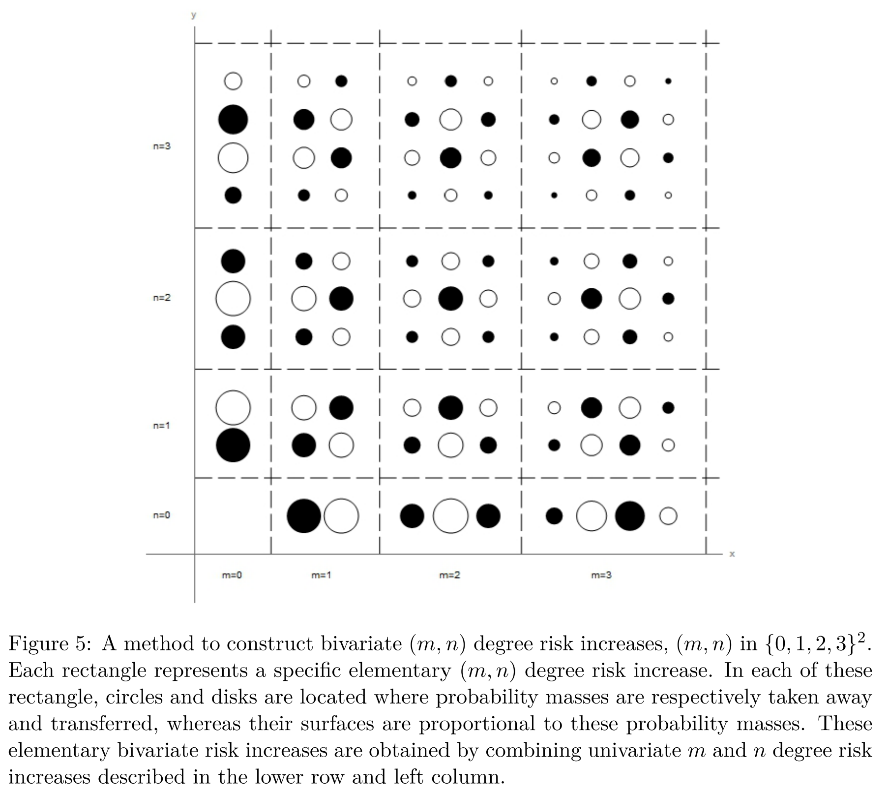
In fact, the right terminology is that the \((m+1)\)-th degree risk aversion describes a preference for the disaggregation of \(m\)-th degree risk increases in \(\tilde x\) with first degree risk increases in \(\tilde y\). Whether m-degree risk increases are perceived as good or bad is irrelevant for defining the \((m+1)\)-degree risk aversion. For example, a prudent person (\(u''' > 0\)) will always dislike increasing the concordance between the second degree riskiness of \(\tilde x\) and the first degree riskiness of \(\tilde y\), independent of whether this person likes or dislikes first and second degree increases in risk.
See earlier drafts of the book!
