Quarto YAML and Markdown: tips and tricks

What I learned today by RTFD.

1 YAML

1.1 This document’s header YAML

---
author: "Stephen J. Mildenhall"
categories:
- meta
- programming
- blog
- Python
date: 2024-02-14
date-modified: 2024-02-21
description: 'What I learned today by RTFD.'
draft: false
title: "Quarto YAML and Markdown: tips and tricks"
toc: true
toc-title: My TOC title
toc-depth: 2
toc-title: Post contents
number-sections: true
number-depth: 2
format:
  html:
    fig-width: 4
    fig-height: 3
image: /static/img/banner-glasses-text-4.png
---

1.2 Project YAML

project:
  type: website
  output-dir: docs
  preview:
    port: 7777

website:
  title: "TestBlog"
  description: "Thoughts and musings on all things Quarto"
  search:
    location: navbar
  navbar:
    background: secondary
    left:
    - about.qmd
    - icon: github
      href: https://github.com/mynl
    - icon: rss
      href: index.xml
  favicon: static/icon/favicon.ico
  site-url: "https://blog.mynl.com"
  twitter-card: true
  open-graph: true

format:
  html:
    theme: litera
    css: styles.css
    smooth-scroll: true
    citations-hover: true
    footnotes-hover: true
    page-layout: full

execute:
  cache: true   # incremental: only recalc if any block changes
  freeze: auto  # re-render only when source changes (global)
  daemon: 600  # stay alive for 600 seconds

1.3 Index YAML

This YAML in ~/index.qmd forces the RSS feed construction.

---
listing:
  contents: posts
  sort: "date desc"
  type: default
  categories: true
  sort-ui: false
  filter-ui: false
  feed:
    categories: [programming, research]
---

2 Basic Cross Referencing

An in-line footnote is ^[footnote text]. A deferred footnote is [^label] followed by [^label]: footnote text elsewhere in the document.

Code

@fig-ug is a map of the ug.  And @fig-line-plot is a line plot.
@fig-balance is the balance and @fig-ug-2 is another underground.

A para of text^[with an inline footnote.]. Inline foot notes are `^[the footnote]`.

A para of text[^a] with a deferred footnote created `text[^a]` and `[a]: below.

@Mildenhall2022 is a fine book. @Pittarello2024 is an AAS work.

[^a]: Here is the actual footnote.

Begets

Figure 4 is a map of the ug. And Figure 1 is a line plot. Figure 5 (b) is the balance and Figure 5 (a) is another underground.

A para of text¹. Inline foot notes are ^[the footnote].

A para of text² with a deferred footnote created text[^a] and `[a]: below.

[1] is a fine book. [2] is an AAS work.

Cross reference reserved prefixes are: fig, tbl, lst, tip, nte, wrn, imp, cau, thm, lem, cor, prp, cnj, def, exm, exr, sol, rem, eq, sec.

Thus

Here is @fig-ug and @Fig-ug. Customize with [my fig @fig-ug] or no prefix with [-@fig-ug].

begets

Here is Figure 4 and Figure 4. Customize with my fig 4 or no prefix with 4.

2.1 Between doc links

You can link between docs with

[about](about.qmd)
[about](about.qmd#section)

Note the qmd extension (works no matter what you render to!)

Seems not to generate auto refs.

Turn off numbering

Use {.unnumbered}.

3 TeX

3.1 Including Macros

Macros can be defined in a hidden block.

::: {.hidden}
$$

\def\RR{{\bf R}}
\def\bold#1{{\bf #1}}

\def\test{Hello, Macro!}

$$
:::

Then, use them:

* $\test$
* $\RR$
* $\bold x$ is a bold x
* Urcorner $x\!\!\urcorner$, $x\!\urcorner$, $x \urcorner$ and $b\!\!\urcorner$, $b\!\urcorner$, $b \urcorner$
* Hence an annuity $\ddot{a}_{x, n\!\urcorner}$

begets

$$

$$

Then, use them:

• \(Hello, Macro!\)
• \({\bf R}\)
• \({\bf x}\) is a bold x
• Urcorner \(x \!\!\urcorner\), \(x \!\urcorner\), \(x \urcorner\) and and \(b\!\!\urcorner\), \(b\!\urcorner\), \(b \urcorner\)
• Hence an annuity \(\ddot{a}_{x, n\!\urcorner}\)

FWIW here is the old lcroof

\def\lcroof#1{
  \hbox{\vtop{\vbox{%
      \hrule\kern 1pt\hbox{%
        $\scriptstyle #1$%
        \kern 1pt}}\kern1pt}%
    \vrule\kern1pt}}

4 Callouts using `div

::: {.border}
This content can be styled with a border
:::

This content can be styled with a border

---

More, the basic callouts:

:::{.callout-note}
Note that there are five types of callouts, including:
`note`, `tip`, `warning`, `caution`, and `important`.
:::

Note

Note that there are five types of callouts, including: note, tip, warning, caution, and important.

4.1 Line breaks

Starting each row with a pipe lets you write poetry.

A line (breaks
  freely, like this)
  persevered

5 Tables

These are standard markdown pipe tables.

| Col1 | Col2 | Col3 |
|------|------|------|
| A    | B    | C    |
| E    | F    | G    |
| A    | G    | G    |

: My Caption {#tbl-letters}

begets

Table 1: My Caption

Col1	Col2	Col3
A	B	C
E	F	G
A	G	G

See Table 1. The label must start with the lbl- prefix. Tables can be nested with divs.

::: {#tbl-panel layout-ncol=2}
| Col1 | Col2 | Col3 |
|------|------|------|
| A    | B    | C    |
| E    | F    | G    |
| A    | G    | G    |

: First Table {#tbl-first}

| Col1 | Col2 | Col3 |
|------|------|------|
| A    | B    | C    |
| E    | F    | G    |
| A    | G    | G    |

: Second Table {#tbl-second}

Main Caption
:::

begets

Table 2: Main Caption

(a) First Table

Col1	Col2	Col3
A	B	C
E	F	G
A	G	G

(b) Second Table

Col1	Col2	Col3
A	B	C
E	F	G
A	G	G

See Table 2 for details, especially Table 2 (b).

6 Executable code blocks

The next code, created using double braces

```{python}
#| echo: fenced
#| label: fig-line-plot
#| fig-cap: "A line plot"

import matplotlib.pyplot as plt
plt.plot([1, 23, 2, 4])
plt.show()
```

begets

```{python}
#| label: fig-line-plot
#| fig-cap: A line plot

import matplotlib.pyplot as plt
plt.plot([1, 23, 2, 4])
plt.show()
```

Figure 1: A line plot

The label is the cross reference, @fig-line-plot = Figure 1.

More options are available. The code

#| label: fig-plots
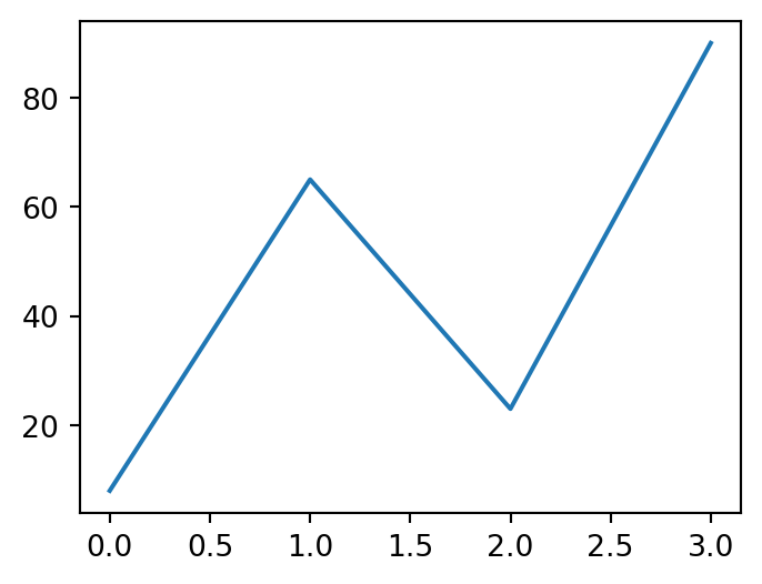
#| fig-cap: "Code and plots a and b"
#| fig-subcap:
#|   - "Listing, suppress with echo: false"
#|   - "Plot a heading"
#|   - "Plot b heading"
#| layout-ncol: 3
#| lst-label: lst-code-block
#| lst-cap: make a test dataframe.

import matplotlib.pyplot as plt
plt.plot([1,23,2,4])
plt.show()

plt.plot([8,65,23,90])
plt.show()

begets

(a) make a test dataframe and plots.

import matplotlib.pyplot as plt
plt.plot([1,23,2,4])
plt.show()

plt.plot([8,65,23,90])
plt.show()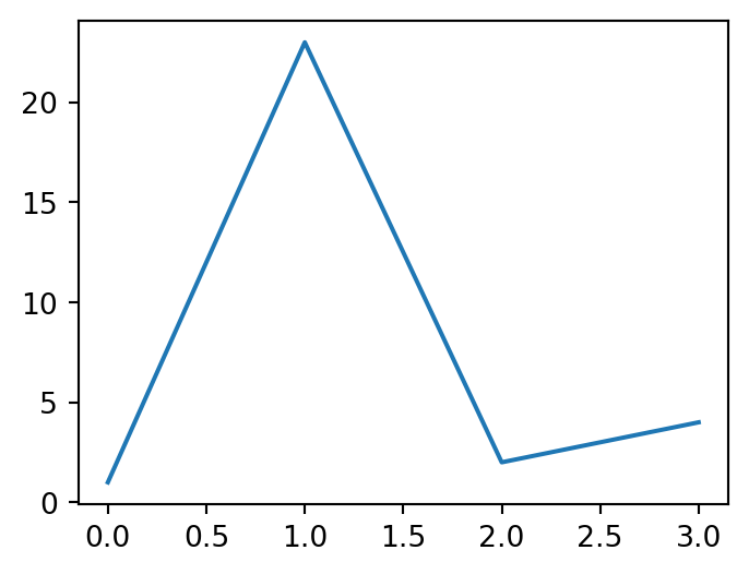

(b) Listing, suppress with echo: false

(c) Plot a heading

Figure 2: Code and plots a and b

The last two lines label the code block listing (hence lst), see #lst-code-block.

See Figure 2 for examples. In particular, Figure 2 (c).

6.1 DataFrame output

The preamble:

#| label: tbl-test
#| tbl-cap: Here is a test dataframe.
#| lst-label: lst-code-block
#| lst-cap: make a test dataframe.

produces output like so. Notice the preamble is stripped from the output.

Listing 1: Listing caption, making a test dataframe.

import pandas as pd
import numpy as np

# this comment remains
df = pd.DataFrame({'x': np.linspace(0,10,21)})
df['y'] = 2. + 3.* df.x
df['z'] = df.x ** 1.3

display(df.iloc[::4])

Table 3: Here is a test dataframe.

	x	y	z
0	0.0	2.0	0.000000
4	2.0	8.0	2.462289
8	4.0	14.0	6.062866
12	6.0	20.0	10.270619
16	8.0	26.0	14.928528
20	10.0	32.0	19.952623

Using just df in the last line, rather than display achieves the same effect:

df.iloc[1::4]

Table 4: Here is a returned test dataframe.

	x	y	z
1	0.5	3.5	0.406126
5	2.5	9.5	3.290956
9	4.5	15.5	7.066043
13	6.5	21.5	11.396916
17	8.5	27.5	16.152681

Listing 1 is a code block listing.

The same kernel runs all code blocks. Hidden code

#| label: tbl-test-3
#| tbl-cap: Here is some of a test dataframe.
#| echo: false

case prints (rather than displays) the table:

Table 5: Here is some of a test dataframe.

       x     y          z
0    0.0   2.0   0.000000
4    2.0   8.0   2.462289
8    4.0  14.0   6.062866
12   6.0  20.0  10.270619
16   8.0  26.0  14.928528
20  10.0  32.0  19.952623

The two tables are Table 3, Table 4 and later Table 5.

6.2 Multiple outputs

As we have already seen, we can make multicolumn output:

#| label: fig-test-3
#| fig-cap: Here is single caption dataframe.
#| fig-subcap:
#|   - "lefthand plot"
#|   - "righthand plot"
#| layout-ncol: 2

begets

ax = df.set_index('x').plot(figsize=(3.5, 2.25))
ax.set(title='mpl title', ylabel='value')

df.plot(figsize=(2.5, 1.5))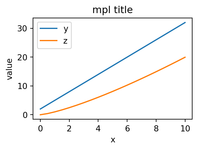

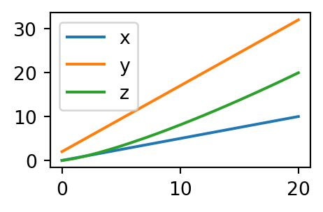
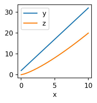
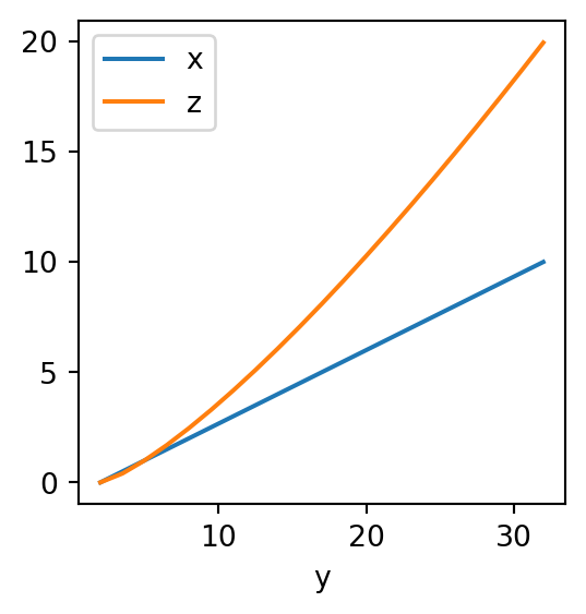
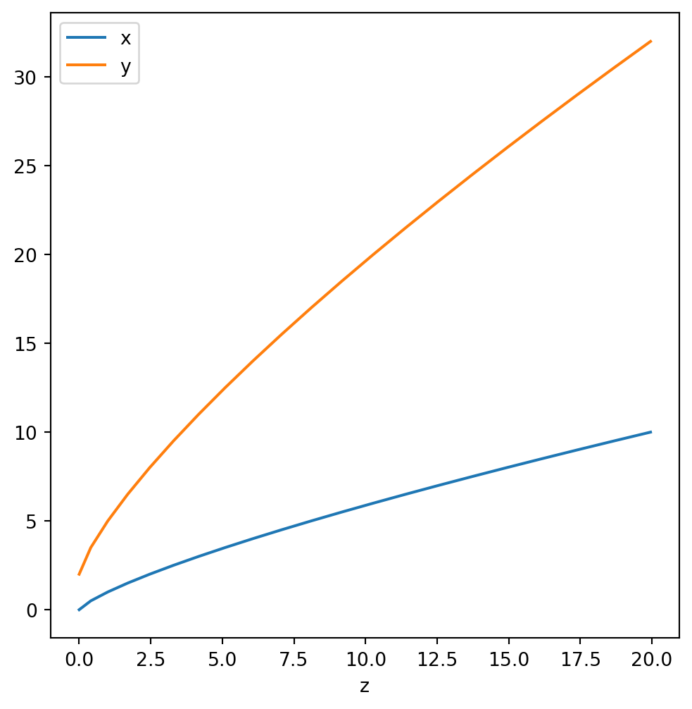
(a) lefthand plot

(b) righthand plot

Figure 3: Here is single caption dataframe.

6.3 Custom Layout

We can make custom plot layouts:

#| layout: [[45,-10, 45], [100]]

df.set_index('x').plot(figsize=(2,2))
df.set_index('y').plot(figsize=(3,3))
df.set_index('z').plot(figsize=(6,6))

interestingly rendered as

::: {#f5616b6c .cell layout='[[45,-10,45],[100]]' execution_count=8}
``` {.python .cell-code}
df.set_index('x').plot(figsize=(2,2))
df.set_index('y').plot(figsize=(3,3))
df.set_index('z').plot(figsize=(6,6))
```

::: {.cell-output .cell-output-display}
![](index_files/figure-html/cell-8-output-1.png){width=196 height=208}
:::

::: {.cell-output .cell-output-display}
![](index_files/figure-html/cell-8-output-2.png){width=269 height=282}
:::

::: {.cell-output .cell-output-display}
![](index_files/figure-html/cell-8-output-3.png){width=492 height=503}
:::
:::

begets

df.set_index('x').plot(figsize=(2,2))
df.set_index('y').plot(figsize=(3,3))
df.set_index('z').plot(figsize=(6,6))

 

6.4 Inline code

If radius is in the kernel, this can work, but not for ipynbs with a cache. It is OK for qmd files.

    The radius of the circle is `{python} radius`

::: {#8204bb91 .cell execution_count=10}
``` {.python .cell-code}
radius = 23.678
```
:::


The radius of the circle is `{python} radius`.

6.5 Four ticks

Can contain pretty much anything.

7 References

Put the references here and not at the end, use refs block:

::: {#refs}
:::

1.

Mildenhall, S.J.: Similar Risks Have Similar Prices: A Useful and Exact Quantification. Insurance: Mathematics and Economics. 105, 203–210 (2022). https://doi.org/10.1016/j.insmatheco.2022.04.006

2.

Pittarello, G., Luini, E., Marchione, M.M.: GEMAct: a Python package for non-life (re) insurance modeling. Annals of Actuarial Science. 1–37 (2024). https://doi.org/10.1017/S1748499524000022

8 Math environments

8.1 Theorems

::: {#thm-line}

### Line

The equation of any straight line, called a linear equation, can be written as:

$$
y = mx + b
$$
:::

begets

Theorem 1 (Line) The equation of any straight line, called a linear equation, can be written as:

\[ y = mx + b \]

See Theorem 1.

::: {.proof}
By induction.
:::

Proof. By induction.

Also thm, lem, cor, prp, def, exm, exr, sol, rem

8.2 Equations

Numbering uses

$$
stuff
$$ {#eq-...}

Black-Scholes (Equation 1) is a mathematical model that seeks to explain the behavior of financial derivatives, most commonly options:

\[ \frac{\partial \mathrm C}{ \partial \mathrm t } + \frac{1}{2}\sigma^{2} \mathrm S^{2} \frac{\partial^{2} \mathrm C}{\partial \mathrm C^2} + \mathrm r \mathrm S \frac{\partial \mathrm C}{\partial \mathrm S}\ = \mathrm r \mathrm C \tag{1}\]

Equation 1 is defined in Section 8.2. Needs number-sections: true to work.

9 Inserting Graphics

9.1 Basic graphic

A figure, width 50% and right aligned:

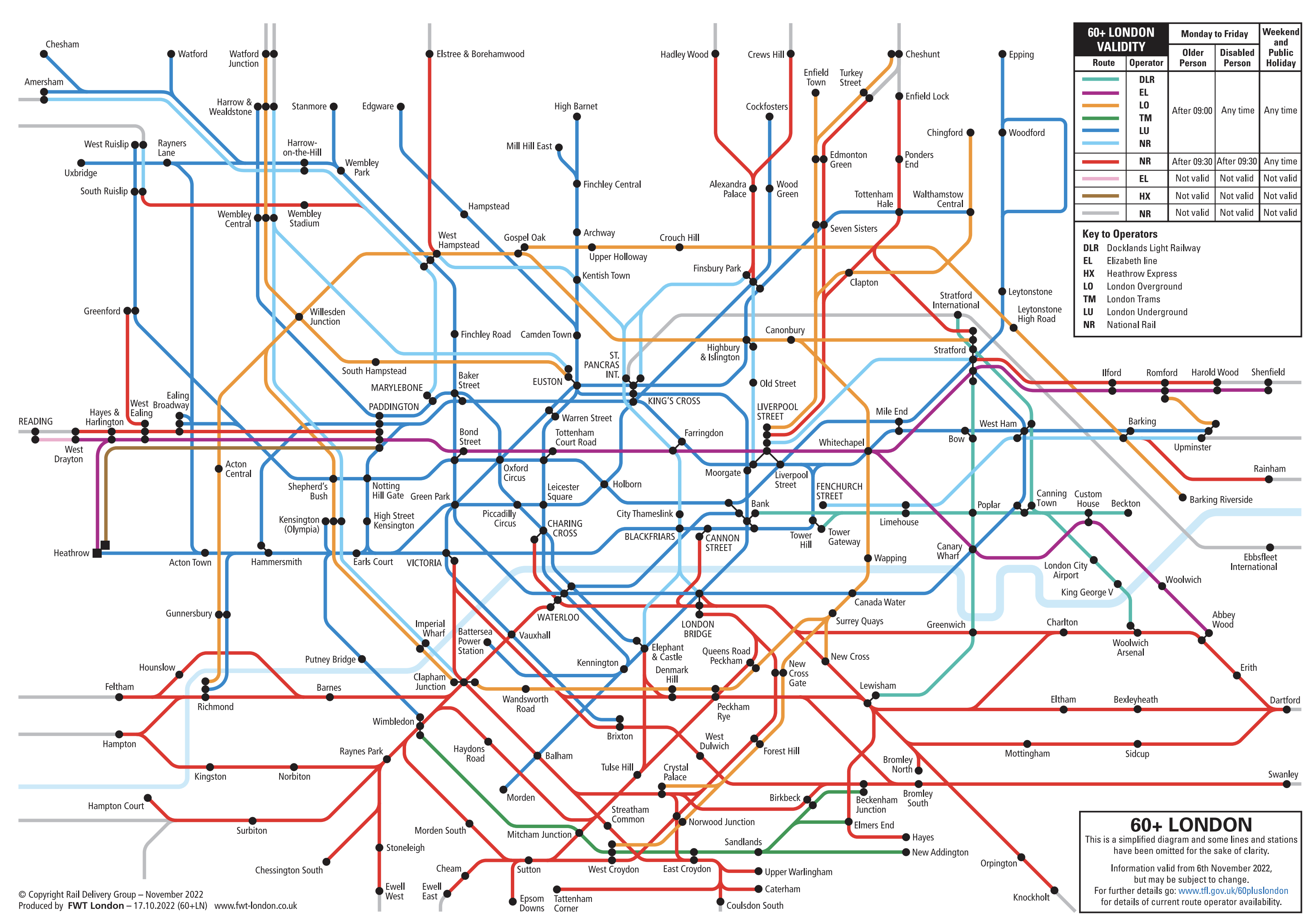![A map of the underground](ug.png){fig-align='right'
width=50% #fig-ug}

Figure 4: A map of the underground

9.2 Side-by-side graphics

Multicolumn output can be arranged with a div. The code

::: {#fig-two-figs layout-ncol=2}

![Underground](ug.png){#fig-ug-2}

![Balance](balance.png){#fig-balance}

Two graphics
:::

begets two side-by-side graphics.

(a) Underground

(b) Balance

Figure 5: Two graphics

10 Customizations

Options like add ins. BTW you can do this https://quarto.org/docs/authoring/cross-reference-options.html to make a link of the link.

11 Execution

11.1 Caching

Caching at the project level with execute: cache: true. If any of the cells in the notebook change then all of the cells will be re-executed. Note that changes within a document that aren’t within code cells (e.g. markdown narrative) do not invalidate the document cache. This makes caching a very convenient option when you are working exclusively on the prose part of a document. Requires the jupyter-cache package (install with pip).

# use a cache (even if not enabled in options)
quarto render example.qmd --cache

# don't use a cache (even if enabled in options)
quarto render example.qmd --no-cache

# use a cache and force a refresh
quarto render example.qmd --cache-refresh

11.2 Freezing

You can use the freeze option to denote that computational documents should never be re-rendered during a global project render, or alternatively only be re-rendered when their source file changes:

execute:
  freeze: true  # never re-render during project render

execute:
  freeze: auto  # re-render only when source changes

Note that freeze controls whether execution occurs during global project renders. If you do an incremental render of either a single document or a project sub-directory then code is always executed.

11.3 Daemons

To mitigate the start-up time for the Jupyter kernel Quarto keeps a daemon with a running Jupyter kernel alive for each document. This enables subsequent renders to proceed immediately without having to wait for kernel start-up.

execute:
  daemon: 600  # stay alive for 600 seconds
  daemon: true

12 Bootstrap classes

Use divs to get to bootstrap:

::: {.grid}
::: {.g-col-4}
This column takes 1/3 of the page
:::
::: {.g-col-8}
This column takes 2/3 of the page
:::
:::

begets

This column takes 1/3 of the page

This column takes 2/3 of the page

Figure 1: A line plot Figure 2 (b): Listing, suppress with echo: false Figure 2 (c): Plot a heading Figure 3 (a): lefthand plot Figure 3 (b): righthand plot Figure 4: A map of the underground Figure 5 (a): Underground Figure 5 (b): Balance

Footnotes

1. with an inline footnote.

2. Here is the actual footnote.